Acknowledgments: Special thanks to Derek Neal for conversations that helped early on in this project. We have benefited greatly from discussions with David Autor, Job Boerma, Jeff Borland, David Deming, James Heckman, Kyle Herkenhoff, Erik Hurst, Francis Kramarz, Guido Menzio and Todd Schoellman, and from the comments of participants at numerous conferences and seminars. We also thank Adam Oppenheimer and Alex Weinberg for their excellent research assistance.
Affiliations: Simon Mongey, Federal Reserve Bank of Minneapolis and NBER.
1 Introduction
Why is there so much wage inequality within occupations? And why has within-occupation wage inequality generally increased over time? Will skill-biased technological change further increase or decrease within-occupation wage inequality? Standard competitive models provide surprisingly little guidance on such questions, even though within-occupation wage inequality is the biggest part of wage inequality. As shown in Table 1, within-occupation inequality accounts for more than two-thirds of the total variance of log wages in the American Community Survey (ACS), and has risen over time.
| Raw | Residual | |||
|---|---|---|---|---|
| Total | Between | Within | Within | controls | |
| 1980 | 0.351 | 0.082 | 0.268 | 0.240 |
| 2010 | 0.407 | 0.121 | 0.286 | 0.270 |
| Change | 0.056 | 0.038 | 0.017 | 0.031 |
Decomposition of the variance of log wages into within- and
between-occupation components using Dorn’s time-consistent occupation
classification (occ1990dd). We report this decomposition
for both raw wages and for
residual wages. Residual wages control for gender,
race and hours with occupation-specific coefficients, hence there is no
remaining between-occupation inequality. Census 1980 and ACS 2010, \(J=290\) three-digit occupations,
employment-weighted by fixed 1980 occupation shares. See Appendix A for further details.
The overall rise in within-occupation wage inequality is modest, but it masks sharp differences across occupations. Figure 1 plots the change in each occupation’s within-occupation inequality from 1980 to 2010 against how intensively it uses cognitive and manual skills. Within-occupation inequality rose most in the most cognitively intensive occupations and fell most in the most manually intensive ones. Why does this divide fall so cleanly between cognitive and manual work?
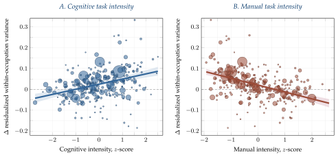
Each point is a three-digit occupation. The vertical axis is the change from 1980 to 2010 in the within-occupation variance of residual log wages with occupation-specific controls for gender, race and hours, as in column 4 of Table 1. Panel A plots this change against the occupation’s cognitive task intensity, Panel B against its manual task intensity, both from Autor and Dorn (2013). Marker area is proportional to 1980 occupation sample size; the solid line is a weighted least-squares fit with its \(95\%\) confidence band. One occupation, farmers, lies below the frame with a change of \(-0.47\); it accounts for \(0.2\%\) of employment and is retained in the estimation. Census 1980 and ACS 2010, \(J = 286\) occupations observed in both years with valid task intensity scores. See Appendix B.1 for more details.
We answer these questions in a general equilibrium model of occupation choice with heterogeneous workers and multiple skills. We find that differences in and changes in skill prices across occupations are key to understanding these facts. In a competitive equilibrium, the wage \(w_{ij}\) that worker \(i\) can earn in occupation \(j\) is linear in their skills \[\tag{1} w_{ij} = \sum_k \, \lambda_{jk} \, x_{ik}\] where \(\lambda_{jk}\) denotes the price of skill \(k\) in occupation \(j\) and \(x_{ik}\) denotes the worker’s endowment of skill \(k\). A key feature of our model is that workers supply their skills as an indivisible bundle. Skill prices \(\lambda_{jk}\) are determined endogenously and may differ across occupations. A given skill may be valued differently in different occupations, depending on the intensity of skill demand across all occupations and the distribution of skill supply. The idea that the bundling of skills in workers creates a constraint on skill supply and the possibility of across-occupation variation in skill prices goes back to Mandelbrot (1962), Rosen (1983) and Heckman and Scheinkman (1987).
Our theoretical contribution is to embed this idea in general equilibrium and determine when the constraint is binding and when it is not, the implications for skill prices across occupations, and their impact on within-occupation wage inequality. We first establish that the competitive equilibrium is constrained efficient, coinciding with the solution to a planning problem in which the bundling of skills appears as a single aggregate constraint. We use this to deliver an interpretation of differences in equilibrium skill prices across occupations in terms of the multiplier on the planner’s bundling constraint. When the constraint is slack, the multiplier is zero and each skill commands a single price across all occupations. A worker earns the same wage whichever occupation they choose. We call this an unbundled equilibrium. When the constraint binds, the multiplier is positive and each skill is priced differently across occupations. We call this a bundled equilibrium. These price differences do not present workers with an arbitrage opportunity: a worker cannot move to the occupation that prices one of their skills more highly without accepting a lower price on their other skills. In a bundled equilibrium, workers with a strong comparative advantage earn rents that shape within-occupation wage inequality.
We then show that our framework nests standard competitive models as limiting cases. Each of these standard models makes use of a stark restriction that shuts down the effects of changes in skill prices on within-occupation wage inequality:
Katz-Murphy — one dimension of skills. The equilibrium is always unbundled. Workers are indifferent between occupations. Within-occupation inequality is the same as overall inequality.
Roy — one priced skill per occupation. The equilibrium is always bundled. Workers sort on comparative advantage. Within-occupation inequality only reflects skills, conditional on selection, and is otherwise independent of skill prices.
One-to-one assignment — one worker type per occupation. Each occupation employs a single type of worker, as in Lindenlaub (2017). Within-occupation inequality is zero.
Our framework relaxes all three restrictions simultaneously. Depending on economic primitives, the competitive equilibrium determines whether skill prices are equated across occupations and, if not, how they vary across occupations.
We then use our framework to derive empirical predictions that can be used to distinguish between three candidate explanations for rising inequality: changing technology, demand, and skill supply. First, a cognitive-biased technology shock is a common, economy-wide increase in the productivity of cognitive skill. The relative price of cognitive skill rises, increasing wage inequality in cognitive-intensive occupations but decreasing wage inequality in manual-intensive occupations. This produces the pattern observed in Figure 1. Our framework further implies that in response to a cognitive-biased technology shock, within-occupation inequality moves primarily through changes in skill prices rather than through changes in skill composition.
By contrast, our framework implies that the other two shocks shape within-occupation inequality primarily through composition, rather than skill prices. A cognitive-biased demand shock is an increase in relative demand for cognitive-intensive occupations. Cognitive occupations expand, drawing in less strongly selected workers, causing within-occupation wage inequality to fall in cognitive-intensive occupations and to rise in manual-intensive ones. This is the opposite of the pattern observed in Figure 1. Finally, a change in the dispersion of cognitive skills can also generate the pattern in Figure 1, again through composition rather than prices, but only if cognitive skills are becoming more dispersed.
We then use US labor market data to evaluate these predictions. We use the NLSY79 with direct measures of workers’ cognitive and manual skills to ask whether a given skill is priced differently across occupations. We use the much larger samples available in the ACS to ask how the prices of education and experience vary across occupations and over time. We establish four main results.
Skills are priced differently across occupations. In the NLSY79, cognitive and manual skill are priced more highly in occupations that use them intensively, and less highly where the other skill is used intensively. Cognitive skill is on average far more valuable than manual skill and its price varies sharply across occupations. Skills are priced as they would be in a bundled equilibrium.
Price differences explain within-occupation inequality across occupations. In the ACS, differences in skill prices across occupations account for the vast majority of the variation in within-occupation inequality associated with observable skills. Differences in composition account for almost none of it.
Price changes over time also explain the rise in within-occupation inequality. From 1980 to 2010, changes in skill prices account for ‘more than all’ of the rise in within-occupation inequality associated with observable skills, and about a third (36%) of the overall rise. Composition, far from driving the rise, worked slightly against it, as the dispersion of education within occupations fell.
The rise is concentrated in cognitive-intensive occupations. The price of education rose most in the occupations that were already most cognitively intensive. About three-fifths of employment is in occupations where the price of education and within-occupation inequality both rose.
Taken together, we find that within-occupation wage inequality is, to a first approximation, a matter of how skills are priced rather than of who works where. Over this period workers within occupations became, if anything, more alike in their skills — the dispersion of education fell, and fell most in the cognitively intensive occupations that had once been the most dispersed of all. On its own, this compression would have reduced within-occupation inequality. The fact that inequality nonetheless rose — and rose precisely where skills became less dispersed — tells us the rise cannot be driven by a changing composition of observable worker skills.
We find that only a cognitive-skill-biased technology shock matches the facts: it raises inequality in cognitive occupations and lowers it in manual occupations, through prices rather than composition. A shift in demand toward cognitive occupations moves inequality the wrong way, and through composition rather than prices.
Generalized Roy models. Our paper builds on a large literature which uses generalizations of Roy (1951) and Heckman and Sedlacek (1985) to study occupational wages and inequality, including Ocampo (2022), Hsieh et al. (2019), Burstein et al. (2019), Böhm (2020), Roys and Taber (2022), and Hurst et al. (2024). Our work is closely related to Erosa et al. (2025), who find that exogenous changes in skill prices account for changes in employment and mean wages since 1980 but play essentially no role in the rise in inequality, which is instead driven by rising within-occupation dispersion in idiosyncratic productivity. In our framework, skill prices vary endogenously across occupations in response to changes in technology, demand, and skill supply, and we find that they play a central role in accounting for wage inequality.
Multidimensional assignment. Our paper also builds on the large literature on multidimensional assignment and sorting, beginning with Becker (1973) and including the one-to-one matching of Lindenlaub (2017) and the many-to-one matching of Eeckhout and Kircher (2018). In these frameworks each firm or job is matched with workers of a single type. Our model has two distinctive features. First, workers of many distinct types sort into the same occupation, giving rise to within-occupation inequality. Second, whether such sorting occurs at all is determined as part of the equilibrium outcome.
Skills bundled in workers. Several recent papers share with us a focus on skill bundles. Choné and Kramarz (2024) and Choné et al. (2024) study related notions of ‘bundling’ and ‘unbundling’ skills. Their notion of unbundling is a fall in the transaction costs of trading skills, which thickens markets. Our notion of unbundling is whether skill prices are equalized across occupations or not in competitive equilibrium, a setting where markets are already thick. Boerma et al. (2025) provide a general theory of comparative statics for technological change in multidimensional assignment models, decomposing its effects into changes in earnings and the reallocation of workers across jobs. Hernnäs (2023) uses a framework similar to ours to study automation.
Skill prices and wage inequality. Our work builds on the large literature which decomposes wage inequality into skill price and composition components, following Lemieux (2006) and Firpo et al. (2011). Like us, Böhm et al. (2024) find, in German administrative data, that skill prices purged of selection help explain rising inequality. Lochner et al. (2025) attribute most of the rise in residual inequality to rising dispersion in unobserved skills.
Skill-biased technical change. Finally, our work relates to the large literature on skill-biased and task-biased technical change, including Bound and Johnson (1992), Juhn et al. (1993), Katz and Murphy (1992), Autor et al. (2008), Autor and Handel (2013), Autor and Dorn (2013), and Deming (2017). A central finding of this literature is that most of the rise in US wage inequality occurred within groups of similar education and experience. Our framework traces this within-group residual to differences in how skills are priced across occupations.
The rest of this paper is organized as follows. Section 2 presents the model. Section 3 establishes constrained efficiency and formalizes the link between the tightness of the planner’s bundling constraint and within-occupation wage inequality. Section 4 shows how standard models are nested as limiting cases. Section 5 derives our key predictions for the roles of skill prices and composition in shaping within-occupation inequality following shocks to technology, demand and skill supply. Section 6 evaluates these predictions in US data, establishing that skills are priced differently across occupations, and quantifying how this accounts for the level and rise of within-occupation inequality. Section 7 concludes.
2 Model
There is a unit mass of workers with heterogeneous endowments of two skills, \(X\) and \(Y\). A homogeneous final good is produced using a set of occupations that are differentially intensive in the different skills.
Skill endowments. Worker \(i\in[0,1]\) has endowments \(x(i)>0\) and \(y(i)>0\) of the two skills. We refer to a worker’s \((x,y)\) pair as their type. Let \(H(x,y)=\text{Prob}[x(i)\leq x,y(i)\leq y]\) denote the distribution of skill types. The associated aggregate endowments are \[\tag{2} \overline{X}:=\int_0^1 \, x(i)\,di,\qquad\text{and}\qquad \overline{Y}:=\int_0^1 \, y(i)\,di\]
Occupations. There are \(j=1,...,J\) occupations. Output \(C_j\) of occupation \(j\) is a constant-returns-to-scale aggregate of the two skills \[\tag{3} C_j = F_j(X_{j},Y_{j})\] The aggregates of skill \(X\) and skill \(Y\) in occupation \(j\) are \[\tag{4} X_{j} = \int_{i\rightarrow j} x(i)\,di,\qquad \text{and} \qquad Y_{j} = \int_{i\rightarrow j} y(i)\,di\] where the notation \(\{i\rightarrow j\}\) denotes the set of workers \(i\) employed in occupation \(j\). The aggregate quantities \(X_j,Y_j\) of skills in occupation \(j\) are the sum of the individual skills of workers assigned to that occupation, i.e., the skills of individual workers are perfect substitutes within a given occupation.
Final good and preferences. The final good is a constant-returns-to-scale aggregate \(U(C_1,...,C_J)\) over the \(J\) occupations. Each worker has linear utility over the final good.
Individual-level bundling constraints. Workers must supply both of their skills to the same occupation. If worker \(i\) chooses occupation \(j\) then worker \(i\) supplies both \(x(i)\) and \(y(i)\) to occupation \(j\). Workers cannot supply \(x(i)\) to one occupation and \(y(i)\) to another. We refer to this collection of restrictions as the individual-level bundling constraints, since they reflect the fact that the skills \(x(i),y(i)\) are physically bundled together in worker \(i\).
We next characterize equilibrium wages in terms of the underlying distribution of skills \(H(x,y)\) and technologies \(F_j(X,Y)\). We do this by first solving a planning problem incorporating the bundling constraints and then establishing that the competitive equilibrium is efficient, allowing us to interpret equilibrium wages using the planning solution.
3 Efficient Allocation and Competitive Equilibrium
In this section we first characterize the efficient allocation and then show that it coincides with the competitive equilibrium. A key insight that simplifies the analysis is that the continuum of individual-level bundling constraints, one for each worker \(i\in[0,1]\), can be summarized by a single aggregate bundling constraint stated in terms of the allocation of aggregate skills \(X,Y\) across occupations. This reformulation leads to a sharp characterization of when skill prices vary across occupations. We focus on the special case of \(J=2\) occupations, which permits a transparent geometric analysis using an Edgeworth box. The extension to general \(J\) is provided in Appendix C.
3.1 Efficient Allocation
The efficient allocation is an allocation of workers to occupations that maximizes final output subject to the production technology and the feasibility constraints, including the constraint that each worker’s skills \(x(i),y(i)\) must be allocated to the same occupation \(j\).
Indirect planning problem. The obvious direct approach to characterizing the efficient allocation would assign each worker \(i\) to an occupation, treating the individual-level bundling constraints explicitly. This introduces a continuum of constraints and associated multipliers, one for each worker. We instead work with an indirect formulation stated in terms of aggregate skills \(X_j,Y_j\) for each occupation \(j\). This reduces the problem to a standard finite-dimensional optimization with a single aggregate constraint. The direct formulation and its equivalence to the indirect formulation are established in Appendix C.
Aggregate bundling constraint. Let \(\mathcal{E}=[0,\overline{X}]\times[0,\overline{Y}]\) denote the Edgeworth box. When skills are indivisibly bundled in workers, the feasible set for the planner is not \(\mathcal{E}\) but rather a subset \(\mathcal{B}\subseteq \mathcal{E}\) that respects the individual-level bundling constraints.
The set \(\mathcal{B}\) is constructed as follows. Begin by ordering workers according to their relative skill endowment \(y(i)/x(i)\) in increasing order. Then, for a given amount of skill \(X\) in occupation 1, ask what is the minimum amount of skill \(Y\) bundled with that \(X\)? This minimum, call it \(\underline{B}(X)\), is obtained by selecting workers starting from those with the lowest \(y/x\) ratios until we reach the required amount \(X\). Likewise, the maximum amount of skill \(Y\) that can be allocated with \(X\), call it \(\overline{B}(X)\), is obtained by selecting workers starting from those with the highest \(y/x\) ratios. The feasible set is then:
\[\tag{5} \mathcal{B}:=\bigg\{ \; (X_1,Y_1)\in \mathcal{E} \; : \; Y_1\in[\,\underline{B}(X_1)\,,\,\overline{B}(X_1)\,]\; \bigg\}\]
Geometrically, \(\mathcal{B}\) is a convex lens in the Edgeworth box, as in Rosen (1983) and Heckman and Scheinkman (1987). The boundaries \(\underline{B}(X)\) and \(\overline{B}(X)\) are increasing in \(X\), i.e., if more skill \(X\) is assigned to occupation 1, more skill \(Y\) must also be assigned. When the distribution \(H(x,y)\) is smooth, the lower boundary \(\underline{B}(X)\) is strictly convex and the upper boundary \(\overline{B}(X)\) is strictly concave. The gradient of the lower boundary is determined by the relative endowment of the marginal worker: \[\tag{6} \underline{B}'(X) = \frac{y(i^*)}{x(i^*)}\] where \(i^*\) denotes the marginal worker when selecting from low to high \(y/x\) to reach a given amount of aggregate skill \(X\).
Intuitively, there are diminishing returns to selecting workers in order of their comparative advantage, giving rise to the convexity of \(\underline{B}(X)\). Starting with workers who have a high comparative advantage in occupation 1, i.e., low \(y\) relative to \(x\), the gradient \(\underline{B}'(X)\) is initially flat — adding a given amount of extra \(X\) brings a small amount of \(Y\) along with it. But as we progress to workers with lower comparative advantage in occupation 1, i.e., high \(y\) relative to \(x\), the gradient \(\underline{B}'(X)\) becomes steeper — the same amount of extra \(X\) now brings a larger amount of \(Y\) along with it.
Example: Fréchet skill distributions. To illustrate these boundaries \(\underline{B}(X),\overline{B}(X)\), suppose skills are independently distributed Fréchet with common shape parameter \(\theta > 1\) \[\tag{7} H_X(x) = \exp\Big(-T_X \, x^{-\theta}\Big), \qquad H_Y(y) = \exp\Big(-T_Y \,y^{-\theta}\Big)\] where the scale parameters \(T_X, T_Y\) are chosen to deliver aggregate endowments \(\overline{X}, \overline{Y}\). For this example, the boundaries of the feasible set work out to be \[\tag{8} \underline{B}(X_1) = \Bigg(1-\left(1 - \left(\frac{X_1}{\overline{X}}\right)^{\frac{\theta}{\theta-1}}\right)^{\frac{\theta-1}{\theta}}\Bigg)\,\overline{Y} ,\qquad \overline{B}(X_1) = \Bigg(1-\left(1-\frac{X_1}{\overline{X}}\right)^{\frac{\theta}{\theta-1}}\Bigg)^{\frac{\theta-1}{\theta}}\overline{Y}\] The shape parameter \(\theta\) controls the dispersion of skills. Lower \(\theta\), closer to 1, implies greater dispersion in skill endowments and produces a wider lens, i.e., the boundaries \(\underline{B}(X)\) and \(\overline{B}(X)\) are farther apart. Higher \(\theta\) implies less dispersion and produces a narrower lens, with the boundaries approaching a straight line from the origin to \((\overline{X}, \overline{Y})\) as \(\theta \to \infty\).
Figure 2 expands on this using a Gaussian copula \(\mathcal{C}\) to control dependence, i.e., \(H(x,y)=\mathcal{C}(H_X(x),H_Y(y))\). Panel A shows individual skills \(x(i), y(i)\) for positive correlation (green) and negative correlation (red). Panel B shows the implied feasible sets \(\mathcal{B}\). When skills are positively correlated, there is a strong pattern of absolute advantage across workers but a weak pattern of comparative advantage — those with high \(x\) also tend to have high \(y\). For a given \(X_1\), worker selection matters little, so the lens is narrow. But when skills are negatively correlated, there is a strong pattern of comparative advantage across workers — those with high \(x\) tend to have low \(y\). Now worker selection matters a lot and the lens is wide.
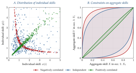
Joint distribution \(H(x,y)=\mathcal{C}(H_X(x),H_Y(y))\) where the marginal distributions are Fréchet with shape parameter \(\theta=1.5\) and the copula is Gaussian with rank correlation \(\tau=\{-0.95,0,+0.95\}\). Panel A shows draws of individual skills \(x(i),y(i)\). Panel B shows the implied feasible sets \(\mathcal{B}\) constraining the aggregate skills \(X,Y\).
Solving the planning problem. With the feasible set \(\mathcal{B}\) in hand, we can state the planning problem in terms of aggregate skills:
Indirect Planning Problem. Choose aggregate skills \(X_j,Y_j\) for \(j=1,2\) to maximize \[\tag{9} U\big(\, F_1(X_1,Y_1)\, , \,F_2(X_2,Y_2)\, \big)\] subject to \[\tag{10} X_{1}+X_{2} \leq \overline{X},\qquad Y_{1}+Y_{2} \leq \overline{Y}\] and the aggregate bundling constraint \[\tag{11} \underline{B}(X_1)\leq Y_1 \leq \overline{B}(X_1)\]
Since \(\underline{B}(X_{1})\) is strictly convex while \(\overline{B}(X_{1})\) is strictly concave, at most one of the bundling constraints binds. Assuming occupation 1 is skill \(X\) intensive, the constraint \(Y_{1}\leq \overline{B}(X_{1})\) is slack. Then let \(\mu\geq0\) denote the multiplier on the remaining constraint \(\underline{B}(X_1)\leq Y_1\). The efficient allocation \(X_1,Y_1\) satisfies the first-order conditions \begin{align} U_1 F_{1X} \,&=\, U_2 F_{2X} \,+\, \mu\, \underline{B}'(X_{1}) \tag{12}\\ U_2 F_{2Y} \,&=\, U_1 F_{1Y} \,+\, \mu\tag{13} \end{align} together with \(X_2 = \overline{X} - X_1\) and \(Y_2 = \overline{Y} - Y_1\).
Bundled and unbundled allocations. The multiplier \(\mu\) determines whether the price of a given skill is equalized across occupations or not. If the bundling constraint is slack, \(\mu=0\), we have an unbundled allocation characterized by a single shadow price for each skill: \(\lambda_X=U_{1} F_{1X}=U_2 F_{2X}\) and \(\lambda_{Y}=U_{2} F_{2Y} = U_{1} F_{1Y}\). The law of one price holds — each skill commands the same price in both occupations. A given worker would be indifferent between occupations, i.e., their shadow price \(\lambda_X x(i) + \lambda_Y y(i)\) is the same regardless of which occupation they work in.
But if the bundling constraint binds, \(\mu>0\), we have a bundled allocation. The bundling constraint creates a gap between skill valuations across occupations. Skill \(X\) is more valuable in occupation 1 than in occupation 2, \(U_1 F_{1X} > U_2 F_{2X}\), while skill \(Y\) is more valuable in occupation 2 than in occupation 1, \(U_2 F_{2Y} > U_1 F_{1Y}\). Workers are sorted into occupations based on their comparative advantage. The shadow price for a worker of type \((x,y)\) in occupation \(j\) is \[\tag{14} \Lambda_j(x,y) = \lambda_{jX}\, x + \lambda_{jY}\, y = U_j \, \big(\,F_{jX} \, x + F_{jY}\,y\,\big)\] where \(\lambda_{jX} = U_j F_{jX}\) and \(\lambda_{jY} = U_j F_{jY}\) are the occupation-specific skill prices. The overall shadow price is \(\Lambda(x,y)=\max_j \Lambda_j(x,y)\), and workers prefer the occupation where their value is highest. Workers with high comparative advantage in their chosen occupation, i.e., those with high \(x/y\) in occupation 1 or high \(y/x\) in occupation 2, earn substantial additional compensation because of the relative scarcity of their skills, scarcity that exists because the bundling constraint binds.
Figure 3 illustrates the two cases. Panel A shows an unbundled allocation where the marginal rate of substitution \(U_1/U_2\) between occupations equals the marginal rate of transformation at a point interior to \(\mathcal{B}\). The allocation satisfies the usual tangency conditions and the bundling constraint is slack. Panel B shows a bundled allocation where the desired tangency point lies outside \(\mathcal{B}\). The allocation is instead found on the boundary \(Y_1=\underline{B}(X_1)\) where the gradient satisfies \[\tag{15} \underline{B}'(X_1) = \frac{U_1 F_{1X}- U_2 F_{2X}}{U_2 F_{2Y} - U_1 F_{1Y}}\]
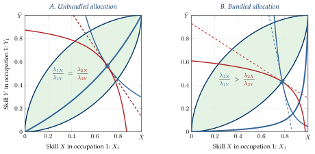
Panel A shows an unbundled allocation where the optimum is at a point interior to \(\mathcal{B}\) satisfying the usual tangency conditions so that skill prices are equalized across occupations, \(\lambda_{1X}/\lambda_{1Y} = \lambda_{2X}/\lambda_{2Y}\). Panel B shows a bundled allocation where the desired tangency point lies outside \(\mathcal{B}\) and the optimum is on the boundary \(\underline{B}(X_1)\), generating a skill price wedge \(\lambda_{1X}/\lambda_{1Y} > \lambda_{2X}/\lambda_{2Y}\).
Figure 4 zooms in on the bundled case to illustrate the geometry when the bundling constraint binds. The planner’s indifference curves are level sets of \(U(F_1(X_1,Y_1),F_2(\overline{X}-X_1,\overline{Y}-Y_1))\) in the Edgeworth box. The bundled allocation \((X_1^b,Y_1^b)\) is found where the planner’s marginal rate of substitution along these indifference curves is equated to the relevant marginal rate of transformation \(\underline{B}'(X_1)\) along the boundary of the aggregate bundling constraint. The curved arrow from \((X_1^b,Y_1^b)\) to the unconstrained allocation \((X_1^u,Y_1^u)\) is the gradient flow, the path of steepest ascent. To reach the unconstrained allocation on the contract curve, the planner would need to reallocate \(X\) from occupation 2 to occupation 1 and \(Y\) from occupation 1 to occupation 2, but this deviation is infeasible — it violates the aggregate bundling constraint.
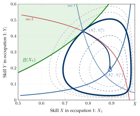
The planner’s indifference curves are level sets of \(U(F_1(X_1,Y_1),F_2(\overline{X}-X_1,\overline{Y}-Y_1))\). The bundled allocation \((X_1^b,Y_1^b)\) is marked with an asterisk where the solid indifference curve is tangent to the boundary \(\underline{B}(X_1)\). The dashed indifference curves are other level sets. The curved arrow from \((X_1^b,Y_1^b)\) to the unconstrained allocation \((X_1^u,Y_1^u)\), marked with an open circle and lying on the contract curve, shows the gradient flow, the path of steepest ascent. The isoquants for each occupation through \((X_1^b,Y_1^b)\) are labeled occ 1 and occ 2; they cross rather than being tangent, reflecting the wedge created by the binding bundling constraint.
3.2 Competitive Equilibrium
We now show that the efficient allocation can be decentralized as a competitive equilibrium.
Final good producers. Let the final good be the numeraire and let \(P_j\) denote the price of output from occupation \(j\). Final good producers maximize profits with technology \(U(C_1,C_2)\), yielding the standard condition \(U_1/U_2=P_1/P_2\).
Occupations. Let \(W_j(x,y)\) denote the wage of a worker with type \((x,y)\) in occupation \(j\). Firms in occupation \(j\) maximize profits with technology \(F_j(X,Y)\). Let \(\lambda_{jX},\lambda_{jY}\) denote the shadow prices of skills \(X,Y\) in occupation \(j\). Cost minimization implies firms hire worker type \((x,y)\) if and only if \(W_j(x,y)\leq \lambda_{jX}\,x+\lambda_{jY}\,y\). Profit maximization then yields \(P_j F_{jX}=\lambda_{jX}\) and \(P_j F_{jY}=\lambda_{jY}\), with zero profits in equilibrium due to constant returns.
Workers. Workers have linear utility over the final good and choose the occupation that maximizes their wage income \(w(i)=\max_j W_j(x(i),y(i))\).
Equilibrium. A competitive equilibrium is a price system \(\{P_j,W_j(x,y)\}\) and allocation \(\{X_j,Y_j\}\) such that firms maximize profits, workers maximize utility, and markets clear.
Our first main result establishes that the competitive equilibrium coincides with the efficient allocation:
Proposition 1. The competitive equilibrium allocation \(X_j, Y_j\) and wages \(W_j(x,y)\) coincide with the efficient allocation and shadow prices from the planning problem. In particular, \(W_j(x,y) = \Lambda_j(x,y)\) for all worker types \((x,y)\) and occupations \(j\).
The significance of this result is that we can use the multiplier \(\mu\) on the aggregate bundling constraint to characterize wage inequality in equilibrium. In equilibrium, workers in occupation \(j\) earn wages \[\tag{16} w_j(i)=\lambda_{jX}\,x(i)+\lambda_{jY}\,y(i)\]
Changes in technologies \(F_j(X,Y)\) or endowments \(H(x,y)\) affect wages both through the usual marginal conditions and through their effects on the bundling multiplier \(\mu\).
3.3 Equilibrium Wage Inequality
Taking the variance of wages within occupation \(j\) then gives \[\tag{17} \text{Var}_j [w(i)] = \lambda_{jX}^2 \,\text{Var}_j[x(i)] \,+\, 2\lambda_{jX}\lambda_{jY}\,\text{Cov}_j[x(i),y(i)] \, + \;\lambda_{jY}^2 \, \text{Var}_j [y(i)]\] In a bundled equilibrium, where skill prices differ across occupations, within-occupation wage inequality will vary across occupations both because of the differences in skill prices and because of the differences in worker skill composition within each occupation, as reflected in the conditional moments — i.e., because of selection. By contrast, in an unbundled equilibrium, skill prices are equalized across occupations, workers earn the same in any occupation \(j\), and wage inequality is the same in every occupation.
Empirical specification. Now suppose that worker skills can be written \((x(i)\varepsilon(i),y(i)\varepsilon(i))\) where \(\varepsilon(i)\) is a worker-level effect independent of \((x(i),y(i))\). Because it multiplies both skills equally, this multiplicative term \(\varepsilon(i)\) has no effect on a worker’s occupational choice, i.e., there is no selection on \(\varepsilon(i)\). Wages are now \(w_j(i)= \big(\lambda_{jX}\,x(i)+\lambda_{jY}\,y(i)\big)\cdot\varepsilon(i)\) so that \(\varepsilon(i)\) captures all the variation in wages not explained by observed skills \((x(i),y(i))\).
Variance of log wages. Our measure of wage inequality will be the variance of log wages. To calculate this we log-linearize within occupation \(j\) to get \[\tag{18} \ln w_j(i) \approx \ln \overline{w}_j + \beta_{jX} \, \ln x(i) + \beta_{jY} \, \ln y(i) + \ln \varepsilon(i)\] where the elasticities \(\beta_{jX},\beta_{jY}\) are weighted averages of the skill prices \(\lambda_{jX},\lambda_{jY}\) \[\tag{19} \beta_{jX}:=\frac{\lambda_{jX}\,\overline{x}_j}{\lambda_{jX}\,\overline{x}_j+\lambda_{jY}\,\overline{y}_j},\qquad \beta_{jY}:=\frac{\lambda_{jY}\,\overline{y}_j}{\lambda_{jX}\,\overline{x}_j+\lambda_{jY}\,\overline{y}_j}\] and where \(\overline{w}_j\), \(\overline{x}_j\) and \(\overline{y}_j\) denote the geometric means of wages and each skill within occupation \(j\). Taking the variance of log wages within each occupation then gives \[\tag{20} \text{Var}_j [\ln w(i)] = \underbrace{\,\boldsymbol{\beta}_j ' \, \boldsymbol{\Sigma}_j \, \boldsymbol{\beta}_j\,}_{=:V_j} + \text{Var}[\ln \varepsilon(i)]\] where \(\boldsymbol{\beta}_j=(\beta_{jX},\beta_{jY})'\) is the vector of equilibrium skill price elasticities and where \(\boldsymbol{\Sigma}_j = \text{Var}_j[(\ln x(i),\ln y(i))]\) is the equilibrium variance-covariance matrix of skills in \(j\).
In our empirical work we will estimate within-occupation wage regressions using both measures of observable worker skills and other controls, such as gender and race. In that setting our focus will be on \(V_j\), the part of within-occupation wage inequality that is attributable to observable skills, and the decomposition of \(V_j\) into (i) a skill price component \(\boldsymbol{\beta}_j\) and (ii) a worker composition component \(\boldsymbol{\Sigma}_j\) reflecting selection on observable skills.
Skill prices and wage inequality. To build intuition for how changes in skill prices change wage inequality, we consider the effect of changes in the skill price gradient \(\lambda_{jX}/\lambda_{jY}\) on the variance of log wages holding worker composition fixed. Since the skill price elasticities \(\beta_{jX}\) and \(\beta_{jY}=1-\beta_{jX}\) are in one-to-one correspondence with the skill price gradient, and the variance of log wages is quadratic in \(\beta_{jX}\) and convex, we then have:
Lemma 1. Within occupation \(j\), the variance \(V_j\) is increasing in the skill price gradient \(\lambda_{jX}/\lambda_{jY}\) if and only if the skill elasticity exceeds the cutoff \[\tag{21} \beta_{jX} > \beta_{jX}^{*} := -\frac{\text{Cov}_j\big[\ln y(i),\ln r(i) \big]} {\text{Var}_j\big[\ln r(i) \big]}\] where \(r(i)=x(i)/y(i)\) is a worker’s comparative advantage in \(X\)-intensive tasks.
The cutoff \(\beta_{jX}^{*}\) depends only on the within-occupation distribution of skills, through a single moment, the (negative of the) within-occupation regression coefficient of a worker’s \(\ln y(i)\) on their comparative advantage \(\ln r(i)=\ln x(i) - \ln y(i)\) in \(X\)-intensive tasks.1
If occupation \(j\) uses skill \(X\) sufficiently intensively, so that \(\beta_{jX}>\beta_{jX}^*\), then changes in technology that increase the relative price of skill \(X\) increase wage inequality within that occupation. Inequality is also more responsive to skill price changes when workers within an occupation have greater dispersion in their comparative advantage, \(\ln r(i)\), as opposed to greater dispersion in either \(\ln x(i)\) or \(\ln y(i)\) separately.
Before explaining our model’s main implications for wage inequality, we first show how our framework nests three standard models as special cases. Importantly, in each of these special cases the model is restricted in a way that shuts down the effects of changes in skill prices on within-occupation wage inequality.
4 Standard Competitive Models Are Limiting Cases
Our framework nests three standard competitive models of skill demand and supply as limiting cases: (i) the (Katz and Murphy 1992) model, (ii) generalized (Roy 1951) models, and (iii) one-to-one competitive assignment models. Each of these makes use of a stark restriction that shuts down the effects of changes in skill prices on within-occupation wage inequality: either there is 1 dimension of skills (Katz-Murphy), 1 priced skill per occupation (Roy), or 1 worker type per occupation (one-to-one assignment).
4.1 Katz-Murphy: One Dimension of Skills
The Katz-Murphy model features a single dimension of worker heterogeneity. In our framework, this is the case where workers vary along only one dimension of skills.
Restricting the skill distribution. To obtain the Katz-Murphy model as a special case, rename the skill aggregates low skill \(L\) and high skill \(H\) and consider technologies \[\tag{22} C_j = F_j(L_j,H_j) \qquad L_j = \int_{i\rightarrow j} l(i)\,di, \qquad H_j = \int_{i\rightarrow j} h(i)\,di\] Now suppose workers are either low-skill workers with type \((l,h)=(l(i),0)\) or high-skill workers with type \((l,h)=(0,h(i))\). That is, each worker has a positive endowment of only one skill. In this setting, the bundling of skills in workers is irrelevant; individuals with one skill do not come bundled with another. This makes the entire Edgeworth box \(\mathcal{E}=[0,\overline{L}]\times[0,\overline{H}]\) feasible, \(\mathcal{B}=\mathcal{E}\). In a sense, workers with orthogonal skill endowments are like ‘Arrow securities’ and the existence of a complete set of Arrow securities makes it possible to span the whole space. Any point in \(\mathcal{E}\) can be obtained by choosing the appropriate combination of low-skill and high-skill workers. Panel A of Figure 5 illustrates.
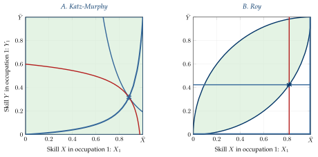
Panel A shows the Katz-Murphy model where workers have orthogonal skill endowments, \((x(i),0)\) or \((0,y(i))\), so the feasible set \(\mathcal{B}\) equals the full Edgeworth box \(\mathcal{E}\) and the equilibrium is always unbundled. Panel B shows the Roy model where the contract curve consists of the bottom and right edges of the box and the equilibrium is always bundled. The lens \(\mathcal{B}\) in Panel B uses independent Fréchet marginals with shape parameter \(\theta=2\).
Always unbundled. Because \(\mathcal{B}=\mathcal{E}\), the aggregate bundling constraint never binds. The equilibrium is always unbundled, regardless of technology. The price of each skill is equalized across occupations: \(\lambda_{1L}=\lambda_{2L}\) and \(\lambda_{1H}=\lambda_{2H}\). Individual workers receive the same wage in both occupations, \(w(i) = \lambda_{L}\,l(i) + \lambda_H\,h(i)\). In particular, low-skill workers earn \(\lambda_L\, l(i)\) and high-skill workers earn \(\lambda_H\, h(i)\), regardless of occupation.
Silent on within-occupation inequality. Shocks to technology shift wages proportionately through the multiplicative skill prices \(\lambda_L,\lambda_H\) alone. The within-occupation variance of log wages remains constant. For example, for low-skill workers \(\text{Var}[\ln w(i)\,|\,j] = \text{Var}[\ln l(i)]\), independent of changes in technology. The Katz-Murphy model is therefore silent on the relationship between changes in technology and within-occupation wage inequality.
4.2 Roy Model: One Skill per Occupation
Where the Katz-Murphy model features a single dimension of skill but multiple inputs in production, the Roy model features a single input in production but multiple dimensions of skill, leading to a meaningful occupational choice problem for workers.
4.2.1 Basic Roy Model
Restricting the technology. The basic Roy model can be obtained as a special case of our framework when the technology in each occupation uses only a single skill, say \(C_1=F_1(X_1)\) and \(C_2=F_2(Y_2)\). While the distribution of skills in the Katz-Murphy model is such that the equilibrium is always unbundled regardless of technology, the technology in the Roy model is such that the equilibrium is always bundled, almost regardless of the distribution of skills.2 Panel B of Figure 5 illustrates. Given the technologies, it would seem natural to assign all of skill \(X\) to occupation 1 and all of skill \(Y\) to occupation 2. But this would place the allocation outside \(\mathcal{B}\), violating the bundling constraints. Instead, the equilibrium is found on the boundary of \(\mathcal{B}\).
Wage levels. In this equilibrium there are only two positive skill prices, \(\lambda_{1X}\) and \(\lambda_{2Y}\). The amounts \(X_2=\overline{X}-X_1\) and \(Y_1=\overline{Y}-Y_2\) are unused and have shadow prices \(\lambda_{2X}=\lambda_{1Y}=0\). Our framework provides an interpretation of wages in the Roy model in terms of the bundling multiplier: \[\tag{23} \lambda_{1X} = \mu\, \underline{B}'(X_1),\qquad \text{and} \qquad \lambda_{2Y} = \mu\] For example, if skills become less dispersed (or more correlated), the feasible set \(\mathcal{B}\) shrinks and the bundling multiplier tightens, increasing both skill prices. This links the dispersion in skills to the level of wages, not just relative wages.3
Silent on within-occupation inequality. Although the equilibrium in the Katz-Murphy model is always unbundled while the equilibrium in the Roy model is almost always bundled, the two models are similarly limited in their ability to speak to within-occupation wage inequality. The common thread is that in both models wages depend on a single factor. In the Roy model, wages are \(w_1(i)=\lambda_{1X}\,x(i)\) for workers in occupation 1 and \(w_2(i)=\lambda_{2Y}\,y(i)\) for workers in occupation 2. The role of technology is limited to selection — the workers in occupation 1 do not represent the full distribution of \(x(i)\) but rather the set of workers who choose to specialize in occupation 1. Apart from these selection effects, the variance of log wages is independent of skill prices and hence independent of technology.
4.2.2 Generalized Roy Model: Many Skills, Two Dimensions
In practice, applied researchers typically work with a version of the Roy model that allows for richer heterogeneity. These generalized Roy models are an important bridge between the basic Roy model and our framework.
Many skills. Let \(\boldsymbol{\xi}(i)\) denote a high-dimensional vector of worker characteristics including cognitive abilities, manual abilities, interpersonal skills, education, experience, and so on. Then suppose that this vector is reduced to two dimensions of skill \[\tag{24} \ln x(i) = \boldsymbol{\xi}(i)'\boldsymbol{a}_{X},\qquad \ln y(i) = \boldsymbol{\xi}(i)'\boldsymbol{a}_{Y}\] The coefficient vectors \(\boldsymbol{a}_X\) and \(\boldsymbol{a}_Y\) map these characteristics into efficiency units for the two skill aggregates \(X\) and \(Y\). This illustrates a key conceptual point: our model permits many skills but restricts attention to two skill dimensions, the sufficient statistics \(x(i)\) and \(y(i)\), for the purposes of production and occupation choice.
Skill prices in generalized Roy vs. our framework. In the generalized Roy model, equilibrium log wages take the form \begin{align} \text{Generalized Roy:}\qquad\ln w_1(i) &= \ln \lambda_{1X}+ \boldsymbol{\xi}(i)'\boldsymbol{a}_{X}\\ \ln w_2(i) &= \ln \lambda_{2Y}+ \boldsymbol{\xi}(i)'\boldsymbol{a}_{Y} \tag{26}\end{align} Skill prices \(\lambda_{1X}\) and \(\lambda_{2Y}\) affect only the intercept, not the slope coefficients on worker characteristics. Within an occupation, the returns to skills are the exogenous technological parameters, \(\boldsymbol{a}_{X},\boldsymbol{a}_{Y}\).
By contrast, in our framework, the returns to underlying skills \(\boldsymbol{\xi}(i)\) are genuinely priced in equilibrium. Log wages are obtained by substituting the technology (24) into the equilibrium wage equation (18) to get \begin{align} \text{Our framework:}\qquad\ln w_1(i) &\approx \ln \overline{w}_1 + \boldsymbol{\xi}(i)'\widetilde{\boldsymbol{a}}_{1},\qquad \widetilde{\boldsymbol{a}}_{1} = \beta_{1X}\boldsymbol{a}_{X}+\beta_{1Y}\boldsymbol{a}_{Y}\tag{27}\\ \ln w_2(i) &\approx \ln \overline{w}_2 + \boldsymbol{\xi}(i)'\widetilde{\boldsymbol{a}}_{2},\qquad \widetilde{\boldsymbol{a}}_{2} = \beta_{2X}\boldsymbol{a}_{X}+\beta_{2Y}\boldsymbol{a}_{Y}\tag{28} \end{align} Shocks that change the equilibrium skill prices \(\lambda_{jX}, \lambda_{jY}\) also change the skill-price elasticities \(\beta_{jX}, \beta_{jY}\), as per (19). Such shocks therefore change not just the intercept but also endogenously re-weight the contributions of underlying skills \(\boldsymbol{\xi}(i)\) to wages, thereby changing within-occupation wage inequality.
Interpretation. This result suggests that standard empirical applications of the generalized Roy model need to be interpreted with care. Researchers who estimate, say, \(\boldsymbol{a}_X\) and \(\boldsymbol{a}_Y\) from wage regressions, often interpret these coefficients as technological parameters. But such wage regressions run on data generated by our model would recover the weighted averages \(\widetilde{\boldsymbol{a}}_1,\widetilde{\boldsymbol{a}}_2\). These coefficients are a mix of the underlying technological parameters \(\boldsymbol{a}_X, \boldsymbol{a}_Y\) and the equilibrium skill prices reflected in \(\beta_{jX}, \beta_{jY}\). Observed variation over time in estimated coefficients may reflect changes in technology, changes in skill prices, or both.
Example: cognitive and manual skills. Suppose \(x(i)\) is an index of a worker’s overall cognitive skill and \(y(i)\) an index of their overall manual skill. Each index is built from underlying cognitive characteristics, manual characteristics, and others \[ \boldsymbol{\xi}(i)=\big(\boldsymbol{\xi}_{\rm cog}(i),\,\boldsymbol{\xi}_{\rm man}(i),\,\boldsymbol{\xi}_{\rm other}(i)\big)\] through the technological coefficients \(\boldsymbol{a}_X\) and \(\boldsymbol{a}_Y\). By construction, a cognitive characteristic increases the cognitive index more than the manual index, so its coefficient in \(\boldsymbol{a}_X\) exceeds its coefficient in \(\boldsymbol{a}_Y\). The same is true in reverse for manual characteristics. From (27), the vector of measured returns to characteristics in occupation \(j\) is the weighted average \[\tag{29} \widetilde{\boldsymbol{a}}_j \;=\; \beta_{jX}\boldsymbol{a}_X+\beta_{jY}\boldsymbol{a}_Y \;=\; \boldsymbol{a}_Y + \beta_{jX}\big(\boldsymbol{a}_X-\boldsymbol{a}_Y\big),\] where the second equality uses \(\beta_{jX}+\beta_{jY}=1\).
Now consider differences in the returns to skills across occupations. Suppose occupations are ordered by cognitive intensity, so that more cognitively intensive occupations have a higher cognitive elasticity \(\beta_{jX}\) — or equivalently, since the two elasticities sum to one, a lower manual elasticity \(\beta_{jY}\). For any characteristic \(k\), the measured return \(\widetilde{a}_j^{\,k} = a_Y^k + \beta_{jX}(a_X^k - a_Y^k)\) is increasing in \(\beta_{jX}\) when \(a_X^k > a_Y^k\) and decreasing otherwise. That is, the measured return rises with cognitive intensity for those characteristics \(k\) that raise a worker’s cognitive skill index \(x(i)\) more than their manual skill index \(y(i)\), and falls with cognitive intensity for those that raise the manual index more. Because higher cognitive intensity means lower manual intensity, the mirror-image statements hold with respect to manual intensity. Overall, we have positive own-intensity gradients — each skill is priced more highly where it is used intensively — together with negative cross-intensity gradients — each skill is priced less highly where the other skill is used intensively.
In a bundled equilibrium, then, this model predicts a \(2\times 2\) set of positive own-intensity and negative cross-intensity gradients. In an unbundled equilibrium, by contrast, \(\beta_{jX}\) is constant across occupations, so \(\widetilde{\boldsymbol{a}}_j\) and hence the return to every characteristic is the same in every occupation, and all four gradients are zero.
4.3 One-to-One Competitive Assignment
Unlike the previous two frameworks, one-to-one competitive assignment models feature heterogeneity in both production and skills along two dimensions. The key difference from our framework is that assignment is one-to-one rather than the many-to-one assignment we emphasize. Our framework is intended to capture the idea that there is considerably more heterogeneity in people than there is heterogeneity in jobs.
Many occupations, one worker per occupation. To make contact with one-to-one assignment models, such as Becker (1973) in one dimension and Lindenlaub (2017) in two dimensions, consider the following version of our setup. Occupations exist on a continuum \(j\in[0,1]\), each associated with a given factor intensity. Factor intensities are continuously distributed with full support on \([0,1]\) and without loss of generality order them from most skill \(X\) intensive, \(j=0\), to least skill \(X\) intensive, \(j=1\). Within each occupation \(j\) is a large number of identical competitive firms. With equal measures of workers and occupations, each worker \(i\) is allocated to a unique occupation \(j^*(i)\), and paid a wage \(w(i) = \lambda_{X}(j^*(i))\,x(i) + \lambda_{Y}(j^*(i))\,y(i)\). Since workers are ordered by comparative advantage and occupations are ordered by skill intensity, the assignment \(j^*(i)\) is increasing, and we write \(i^*(j)\) for its inverse, the worker in occupation \(j\).4
No within-occupation inequality. Since each occupation is assigned a unique type of worker, there is again no notion of within-occupation inequality. All workers in a given occupation are identical by construction. In a one-to-one matching model all workers are marginal; there are none of the inframarginal rents that determine within-occupation inequality in our benchmark model.
Aggregate bundling constraints with many occupations. As in the Roy model, expressing the planning problem in terms of the aggregate bundling constraints yields an intuitive characterization of skill prices. For any occupation \(j\), the allocation of workers to occupations \(j'<j\) must be feasible given the distribution of skills. Let \(X^{(j)}:=\int_0^j X(j')\,dj'\) and \(Y^{(j)}:=\int_0^j Y(j')\,dj'\) denote the cumulative skills allocated to occupations \([0,j]\), where \(X(j)\) and \(Y(j)\) denote the skills employed in occupation \(j\). As shown in Appendix C.2, we can express the problem in terms of a continuum of aggregate bundling constraints of the form \[\tag{30} Y^{(j)} \geq \underline{B}\big(X^{(j)}\big),\qquad \text{for all $j\in[0,1]$}\] where \(\underline{B}(X)\) is the same lower boundary function as in the two-occupation case, with multiplier \(\mu(j)\geq0\), and which binds at every \(j\) when the sorting is one-to-one. In short, the cumulative skill \(Y\) allocated to occupations \([0,j]\) must be consistent with the cumulative skill \(X\) allocated to those occupations.
The equilibrium conditions between adjacent occupations can then be written \[\tag{31} \frac{d\lambda_{X}(j)}{dj} = -\mu(j)\left(\frac{y(i^\ast(j))}{x(i^\ast(j))}\right), \qquad \frac{d\lambda_{Y}(j)}{dj} = \mu(j)\] so that, moving toward less skill \(X\) intensive occupations, the price of skill \(X\) falls and the price of skill \(Y\) rises, and both do so only where the bundling constraint binds. Integrating the first of these from the most skill \(X\) intensive occupation, \(j=0\), up to any \(j\) delivers: \[\tag{32} \lambda_{X}(j) = \lambda_{X}(0) - \int_0^j {\mu}(j') \left(\frac{y(i^\ast(j'))}{x(i^\ast(j'))}\right) \,dj'\] where \(\lambda_{X}(0)\) is the marginal product of skill \(X\) in the most skill \(X\) intensive occupation, evaluated at the worker type \(i=0\) with the highest \(x(i)/y(i)\) ratio. The price of skill \(Y\) is the mirror image, rising from \(\lambda_Y(0)\) by the accumulated multipliers \(\int_0^j\mu(j')\,dj'\).
The price of skill \(X\) in occupation \(j\) equals its price in the most skill \(X\) intensive occupation, \(j=0\), minus an adjustment reflecting the tightness of the bundling constraints in less skill \(X\) intensive occupations. For example, if skills became less diverse, these constraints would tighten, leading to a steeper profile of skill prices across occupations. Less diverse skills would lead to lower economy-wide wage inequality (because there are fewer extreme types), while steeper gradients of skill prices would lead to greater dispersion in wages across occupations.
We have now established that three leading competitive models are silent on the relationship between technology and within-occupation inequality. The Katz-Murphy model restricts worker heterogeneity to one dimension, the generalized Roy model restricts production to one priced skill per occupation, and one-to-one assignment models restrict each occupation to one worker type. Our framework relaxes all three restrictions simultaneously, permitting multiple skill dimensions, multiple skills per occupation, and multiple worker types per occupation. We now turn to the central question these models cannot address: how do changes in the economic environment affect wage inequality within occupations?
5 Skill Prices and Wage Inequality
In this section we characterize how changes in the tightness of the bundling constraint shape the prices of skills within and across occupations, and thereby wage inequality. Section 5.1 provides analytical results precisely characterizing the tightness of the bundling constraint and the implications for skill prices and wage inequality. Section 5.2 uses these results to deliver predictions for the impact of changes in technology, demand, and skill supply on skill prices, worker composition, and wage inequality.
5.1 When Is the Bundling Constraint Tight?
We first provide analytical results characterizing the tightness of the bundling constraint and its implications for skill prices. We assume that occupation-level technologies are Cobb-Douglas in aggregate skills and that worker-level skills are distributed IID Fréchet with a common shape parameter. For this setting we give an exact condition on parameters determining whether the equilibrium is bundled or not. We then specialize further to a perfectly symmetric economy, where we can characterize how tightly the constraint binds, and show how increases in factor intensity tighten the bundling constraint, increasing the bundling multiplier and the return to the skill each occupation uses most intensively.
5.1.1 Cobb-Douglas-Fréchet
Suppose that occupation-level output is Cobb-Douglas in aggregate skills \[\tag{33} C_j = X_j^{\alpha_j}\, Y_j^{1-\alpha_j}\qquad j=1,2\] where \(\alpha_j\in(0,1)\) is a measure of factor intensity. To simplify the exposition we assume \(\alpha_1>\alpha_2\) and refer to \(X\) as the primary skill for occupation 1 and \(Y\) as the primary skill for occupation 2. We also assume that the final good is Cobb-Douglas in occupations \[\tag{34} U(C_1,C_2) = C_1^{\eta_1} C_2^{\eta_2}\] with \(\eta_1+\eta_2=1\) denoting the shares of each occupation in final output.
Unbundled allocation. If the bundling constraint is slack, \(\mu=0\), we can solve the system of first order conditions (12)-(13) to get the allocations \[\tag{35} X_1 = \frac{\eta_1 \alpha_1}{\eta_1 \alpha_1 + \eta_2 \alpha_2}\, \overline{X}, \qquad \qquad Y_1 = \frac{\eta_1 (1-\alpha_1)}{\eta_1 (1-\alpha_1) + \eta_2 (1-\alpha_2)} \, \overline{Y}\] along with \(X_2=\overline{X}-X_1\) and \(Y_2=\overline{Y}-Y_1\). But is this allocation feasible?
When is the equilibrium bundled? The unbundled allocation is infeasible when the underlying demand for primary skills cannot be accommodated by the available composition of skill supply. One version of this is that the equilibrium will be bundled if the weight on primary skills in each occupation is sufficiently high. To check if the unbundled allocation is feasible, we evaluate the aggregate bundling constraint \(Y_1\geq \underline{B}(X_1)\) at this allocation. When \(\alpha_1\) increases, the constraint will at some point be violated: \(Y_1\) monotonically decreases, while \(X_1\) monotonically increases and hence \(\underline{B}(X_1)\) increases. Hence there is a unique \(\alpha_1^\ast\) such that the equilibrium is bundled if and only if \(\alpha_1\geq \alpha_1^*\). A pure Roy economy is the limit \(\alpha_1=1\), \(\alpha_2=0\) where the equilibrium is always bundled.
A second version of this is that the equilibrium will be bundled if the dispersion in skills is sufficiently low. Plugging the unbundled allocations into the bundling constraint under IID Fréchet skills (8), we obtain: \[\tag{36} Y_1\geq \underline{B}(X_1) \, \Longleftrightarrow \, \bigg\{\bigg(\underbrace{\frac{\eta_1 \alpha_1}{\eta_1 \alpha_1 + \eta_2 \alpha_2}}_{\text{unbundled $X_1/\overline{X}$}}\bigg)^{\frac{\theta}{\theta-1}} + \bigg(\underbrace{\frac{\eta_2 (1-\alpha_2)}{\eta_1 (1-\alpha_1) + \eta_2 (1-\alpha_2)}}_{\text{unbundled $Y_2/\overline{Y}$}}\bigg)^{\frac{\theta}{\theta-1}}\bigg\}^{\frac{\theta-1}{\theta}} \leq 1\] where \(\theta>1\) is the Fréchet shape parameter. If \(X_1/\overline{X}\) and \(Y_2/\overline{Y}\) are high, the economy wants a more specialized allocation of primary skills. This is only possible if there is sufficient skill diversity. As \(\theta\rightarrow\infty\) skill diversity decreases and the left side of the constraint approaches \(X_1/\overline{X}+Y_2/\overline{Y}\), which exceeds 1, so the equilibrium is bundled. Hence there is a unique \(\theta^\ast\) such that the equilibrium is bundled if and only if \(\theta\geq\theta^\ast\). A Katz-Murphy economy is the opposite limit \(\theta\rightarrow1\) where skill diversity is high and the equilibrium is always unbundled.
For a given configuration of parameters, we now know whether the equilibrium is bundled or not. To understand equilibrium skill prices and wage inequality, we next specialize to a symmetric economy, where we can characterize how tightly the bundling constraint binds. We show that an increase in the intensity with which an occupation uses its primary skill tightens the bundling constraint, increasing the bundling multiplier, the relative price of that skill, and wage inequality.
5.1.2 Symmetric Economy
In a symmetric economy we can calculate the equilibrium bundling multiplier, skill prices, and within-occupation inequality in closed form. We maintain IID Fréchet worker-level skills with common shape parameter \(\theta>1\) and add the following symmetry condition:
Symmetric Economy. The occupation-level technologies are mirror images of each other, \(\alpha:=\alpha_1=1-\alpha_2\geq1/2\). Occupations have equal expenditure shares in final output, \(\eta_1=\eta_2=1/2\), and the aggregate amounts of each skill are the same, \(\overline{X}=\overline{Y}\).
With this, each occupation receives an equal quantity of its primary skill, \(X:=X_1=Y_2\), and an equal quantity of its secondary skill, \(X_2=Y_1=\overline{X}-X\), so the aggregate allocation is summarized by just \(X\). When the bundling constraint is slack, this allocation is simply \(X(\alpha)=\alpha\overline{X}\). When it binds, \(X\) is capped at a level \(X^*(\theta)\) determined by the bundling constraint alone — independent of the technology, and in particular independent of \(\alpha\).
This economy is indexed by two parameters: the intensity \(\alpha\geq1/2\) which governs how strongly the economy wants to specialize in primary skills, and the dispersion \(\theta>1\), which governs the shape of the feasible set \(\mathcal{B}\) and hence how much of that want can be met before the bundling constraint binds. To simplify notation we suppress the dependence of equilibrium outcomes on \(\theta\). We then have:
Proposition 2 (Symmetric equilibrium). For any symmetric economy:
There is a unique primary skill intensity \[\tag{37} \alpha^* = \left(\frac{1}{2}\right)^{\frac{\theta-1}{\theta}}\] such that the equilibrium is unbundled if and only if \(\alpha\leq\alpha^*\).
The equilibrium allocation of the primary skill is \[\tag{38} X(\alpha) =\left\{\begin{array}{rcl} \alpha \overline{X} &\hspace{0.1cm}& \alpha\leq \alpha^* \\[0.3cm] \alpha^* \overline{X} &\hspace{0.1cm}& \alpha>\alpha^* \end{array}\right.\]
The equilibrium bundling multiplier is \[\tag{39} \mu(\alpha) =\left\{\begin{array}{ccl} 0 &\hspace{0.1cm} & \alpha\leq \alpha^* \\[0.3cm] \dfrac{1}{2}\left(\dfrac{\alpha^{*}}{1-\alpha^{*}}\right)^{\alpha}\left(\dfrac{\alpha-\alpha^{*}}{\alpha^{*}}\right) &\hspace{0.1cm} & \alpha>\alpha^* \end{array}\right.\]
Implications for allocations. The intuition is straightforward. An increase in the primary-skill intensity \(\alpha\) increases demand for the primary skill. When the equilibrium is unbundled, this demand is met by reallocating workers across occupations, and the primary-skill allocation \(X(\alpha)=\alpha \overline{X}\) increases with \(\alpha\). But eventually the allocation hits the ceiling \(X^*(\theta)\) so that \(X(\alpha^*)=X^*(\theta)\). Once \(\alpha\) reaches \(\alpha^*\) the bundling constraint binds, the allocation is stuck at \(X^*(\theta)\), and further increases in \(\alpha\) no longer change the allocation but instead tighten the constraint — the multiplier \(\mu(\alpha)\) increases with the gap \(\alpha-\alpha^*\). The more intense the economy’s unfulfilled demand for primary skill, the tighter the bundling constraint and the larger the premium on a unit of primary skill in its primary occupation.
Implications for skill prices. When the equilibrium is unbundled, \(\alpha\leq\alpha^*\), an increase in \(\alpha\) is absorbed through quantity adjustments — an increase in \(X(\alpha)\) — with no change in relative skill prices. When the equilibrium is bundled, \(\alpha>\alpha^*\), the allocation cannot adjust and the shock is instead absorbed through prices. In a symmetric equilibrium, relative skill prices are \[\tag{40} g(\alpha):=\dfrac{\lambda_{1X}}{\lambda_{1Y}}= \dfrac{\lambda_{2Y}}{\lambda_{2X}} =\left\{\begin{array}{cc} 1 & \alpha\leq \alpha^* \\[0.3cm] \left(\dfrac{\alpha}{1-\alpha}\right) \bigg/ \left(\dfrac{\alpha^*}{1-\alpha^*}\right) & \alpha>\alpha^* \end{array}\right.\] In an unbundled equilibrium, each skill has the same price across occupations, and, by symmetry, the two skills command the same price within an occupation, leading to a relative price of \(g(\alpha)=1\). In a bundled equilibrium, the primary skill is relatively scarce in its primary occupation and receives a premium. This bundling multiplier \(\mu(\alpha)\) is this premium. Under symmetry it is both the across-occupation wedge in each skill’s price and the within-occupation gap between the two skill prices, \[ \mu = \underbrace{\,\lambda_{1X} - \lambda_{2X}\,}_{\text{across-occupations}} \,=\, \underbrace{\,\lambda_{1X} - \lambda_{1Y}\,}_{\text{within-occupation}}\] so the relative skill price is \(g=1+\mu/\lambda_{1Y}>1\). Notice that greater skill dispersion, lower \(\theta\), increases \(\alpha^*\) and so reduces the primary-skill premium in a bundled equilibrium.
Implications for wage inequality. We can use this result to connect the primary-skill intensity \(\alpha\) to within-occupation wage inequality. Recall the primary-skill elasticity \(\beta_{1X}\), from (19), which can be written in terms of the relative price of the primary skill and the relative quantity of the primary skill among the workers who select into the occupation \[\tag{41} \beta_{1X} = \frac{\dfrac{\lambda_{1X}}{\lambda_{1Y}} \cdot \left(\dfrac{\overline{x}_1}{\overline{y}_1}\right)}{\dfrac{\lambda_{1X}}{\lambda_{1Y}} \cdot \left(\dfrac{\overline{x}_1}{\overline{y}_1}\right)+1}\] Under symmetry the relative skill price is \(g(\alpha)\) and the relative quantity, in both occupations, works out to be \(\overline{x}/\overline{y}=4^{1/\theta}\), the geometric mean comparative advantage when skills are IID Fréchet with common shape parameter \(\theta\). So under symmetry we can write \[\tag{42} \beta(\alpha) := \frac{g(\alpha) \cdot 4^{1/\theta}}{g(\alpha)\cdot 4^{1/\theta}+1} \geq \frac{1}{2}\] Since \(\beta(\alpha)\geq1/2\), equilibrium wages are more responsive to the primary skill than to the secondary skill. In an unbundled equilibrium, \(g(\alpha)=1\) and the elasticity is a constant pinned down by \(\theta\) alone.
We can then write the variance of log wages, common to both occupations \[\tag{43} V(\alpha) = \Big(\,\kappa_0 + \kappa_1\,\beta(\alpha) + \kappa_2\,\beta(\alpha)^2\,\Big)\cdot \frac{1}{\theta^2}\] where the coefficients \(\kappa_0\), \(\kappa_1\) and \(\kappa_2\) are numerical constants that do not depend on \(\alpha\) or \(\theta\).5
Within-occupation inequality depends on the intensity \(\alpha\) only through the skill-price gradient \(g(\alpha)\) — the price channel — as it enters \(\beta(\alpha)\), while the dispersion of worker skills \(\theta\) shapes the composition of wages conditional on selection — the composition channel. We will measure these two channels in US data below. The variance is increasing in \(\beta(\alpha)\) if and only if \(\beta(\alpha)>\beta^*\), the critical elasticity from Lemma 1, which works out to be \[\tag{44} \beta^* = - \frac{\kappa_1}{2\kappa_2} \approx 0.149\] Since the equilibrium elasticity \(\beta(\alpha)\geq 1/2>\beta^*\), we are always on the increasing arm of the quadratic. In a bundled equilibrium, an increase in \(\alpha\) steepens the gradient \(g(\alpha)\), increasing the elasticity \(\beta(\alpha)\) and increasing inequality. Hence:
Proposition 3 (Symmetric wage inequality). For any symmetric economy:
In an unbundled equilibrium, \(\alpha\leq \alpha^*\), the variance of log wages is a constant \(\overline{V}\), independent of the primary-skill intensity \(\alpha\).
In a bundled equilibrium, \(\alpha>\alpha^*\), the variance of log wages \(V(\alpha)\) is strictly increasing in \(\alpha\), with \(V(\alpha^*)=\overline{V}\).
This is a stark result. If the equilibrium is unbundled, within-occupation inequality is completely flat — independent of \(\alpha\), at a level \(\overline{V}\) set by the dispersion of worker skills. Inequality begins to increase with \(\alpha\) precisely when \(\alpha\) crosses \(\alpha^*\) and the equilibrium becomes bundled. It is the steepening of the skill-price gradient \(g(\alpha)\), as the constraint tightens, that raises the return to the primary skill and with it within-occupation inequality.
More general CES technologies. The closed-form results above are specific to Cobb-Douglas technologies, but the same patterns hold under more general symmetric CES technologies, as shown in Figure 6. We consider symmetric economies from \(\alpha=1/2\) to \(\alpha=1\). Panel A shows the feasible set \(\mathcal{B}\) and the contract curves as \(\alpha\) increases. At \(\alpha=1/2\) the allocation \(X(\alpha)\) is interior to \(\mathcal{B}\) and the equilibrium is unbundled with \(\mu(\alpha)=0\). As \(\alpha\) increases, \(X(\alpha)\) increases — with the allocation moving southeast in the Edgeworth box — until it reaches the boundary \(\underline{B}(X)\), determining \(\alpha^*\). For \(\alpha>\alpha^*\) the allocation remains fixed at \(X(\alpha^*)\) while the multiplier \(\mu(\alpha)\) increases, as shown in Panel B. Within-occupation wage inequality increases with \(\alpha\) in the bundled region, as shown in Panel C.
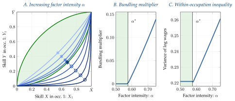
Panel A shows the feasible set \(\mathcal{B}\) and contract curves as factor intensity \(\alpha\) increases, with asterisks marking the equilibrium allocation. For \(\alpha \leq \alpha^*\) the equilibrium is unbundled and the allocation moves southeast. For \(\alpha > \alpha^*\) the equilibrium is bundled at the boundary \(\underline{B}(X_1)\) (fixed asterisk \(\boldsymbol{*}\)) while the unconstrained optimum drifts further outside \(\mathcal{B}\) (open circles \(\circ\)). Panel B shows the bundling multiplier \(\mu(\alpha)\), zero in the unbundled region and increasing in the bundled region. Panel C shows the within-occupation variance of log wages, flat for \(\alpha \leq \alpha^*\) and rising for \(\alpha > \alpha^*\). The green shaded region indicates \(\alpha \leq \alpha^*\). Parameters: independent Fréchet marginals with \(\theta = 2.25\), CES production with \(\sigma = 0.60\), symmetric economy with \(\eta_1 = \eta_2 = 0.5\) and \(\overline{X}=\overline{Y}\).
With these symmetric analytics in hand, we now turn to applications of our framework in asymmetric settings that, while stylized, more closely resemble the differences in occupational structure that we will see in our empirical work. In particular, we show how to interpret differences in within-occupation inequality between cognitive-intensive and manual-intensive occupations in response to cognitive-biased changes in technology, shifts in the composition of final demand, and changes in skill dispersion.
5.2 Understanding the Rise in Within-Occupation Inequality
We now ask what economic forces in our model can explain the observed long-run rise in within-occupation wage inequality and the differences in inequality between cognitive-intensive and manual-intensive occupations. We consider three candidate explanations: (i) cognitive-biased technological change that increases the productivity of cognitive skills in all occupations, (ii) cognitive-biased shifts in demand, and (iii) changes in the dispersion of cognitive skill. Each generates changes in relative skill prices across occupations and changes in worker composition across occupations, including through selection. We compute the variance of log wages for each occupation, \(V_j\), and decompose this into the component attributable to changes in relative skill prices and the component attributable to changes in composition.
For expositional simplicity we continue to focus on the case of \(J=2\) occupations but we also present numerical results for general \(J\geq 2\) occupations when having more occupation-level variation makes the empirical content of the results more transparent. Throughout we assume that occupation-level production is CES in aggregate skills and final output is Cobb-Douglas in occupation output. We continue to assume that skills are independent Fréchet \(H(x,y)=H_X(x)H_Y(y)\) but with potentially distinct marginals.
CES in cognitive and manual skills. Suppose that occupation-level output is \[\tag{45} F_j(X_j,Y_j) = \Big[\, \alpha_j (A_X X_j)^{\sigma} + (1-\alpha_j) (A_Y Y_j)^{\sigma}\,\Big]^{1/\sigma},\qquad j=1,2\] where \(A_X\) and \(A_Y\) are skill-augmenting productivity levels, common across occupations, and \(\tfrac{1}{1-\sigma}\) is the elasticity of substitution between aggregate skills. For the following applications we refer to \(X\) as cognitive skill and to \(Y\) as manual skill. The factor intensities \(\alpha_j\) are occupation-specific but we no longer impose symmetry. We continue to assume \(\alpha_1\geq 1/2 \geq \alpha_2\) so that occupation 1 is relatively intensive in cognitive skill and occupation 2 is relatively intensive in manual skill.
5.2.1 Cognitive-Biased Technological Change
We first consider a uniform increase in the productivity \(A_X\) of cognitive skills. Occupations respond differently to this common shock because of their differences in cognitive intensity, \(\alpha_j\). In particular, we find that this common shock can generate diverging trends in within-occupation wage inequality, with inequality rising in the cognitive-intensive occupations and falling in the manual-intensive occupations. In this sense, the model is capable of rationalizing the diverging long-run trends in within-occupation wage inequality documented in Figure 1.
Contract curve invariant to \(A_X\). To understand the effects of an increase in \(A_X\) we begin with the unbundled allocation. As usual, this is found on the contract curve where the marginal rates of technical substitution \(F_{jX}/F_{jY}\) are equalized across occupations \(j\). But the common \(A_X\) shock shifts \(F_{jX}/F_{jY}\) in both occupations equally, leaving the contract curve itself unchanged. If the elasticity of substitution \(\tfrac{1}{1-\sigma}\) between skills \(X\) and \(Y\) is greater than the elasticity of substitution between occupation-level outputs \(C_1\) and \(C_2\) in final output, the allocation shifts down and to the left along the contract curve as \(A_X\) increases. Otherwise it shifts up and to the right. Panel A of Figure 7 illustrates. In this example the skills \(X\) and \(Y\) are substitutes, \(\tfrac{1}{1-\sigma}>1\), and since the Cobb-Douglas final good aggregator is unit-elastic the allocation shifts down and to the left.
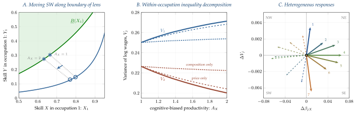
Panel A shows the feasible set \(\mathcal{B}\), with the lower boundary \(\underline{B}(X_1)\) and the contract curve as cognitive productivity \(A_X\) rises from \(1\) to \(2\). Asterisks (\(\boldsymbol{*}\)) mark the bundled equilibrium, open circles (\(\circ\)) mark the unconstrained optimum on the contract curve. Panel B shows the within-occupation variance of log wages \(V_j\) for each occupation, decomposed into a price component (dashed, holding composition fixed) and a composition component (dotted, holding prices fixed). Panel C plots the change in cognitive skill price elasticity \(\Delta\beta_{jX}\) against the change in its within-occupation inequality \(\Delta V_j\) for \(J=7\) occupations, with points numbered and colored from \(j=1\), the most cognitive-intensive, to \(j=7\), the most manual-intensive. Solid arrows show the response to the cognitive productivity shock \(A_X\). Dashed arrows show the mirror-image response to a manual productivity shock \(A_Y\). Parameters: independent Fréchet marginals with \(\theta = 2.25\), CES production with \(\sigma = 0.60\), symmetric economy with \(\eta_1 = \eta_2 = 0.5\) and \(\overline{X}=\overline{Y}\).
Quantity responses are dampened in a bundled equilibrium. Now consider a bundled equilibrium, with an initial allocation on the boundary of \(\mathcal{B}\), not the contract curve. Then as shown in Panel A, an increase in \(A_X\) leads to a similar but smaller change in the allocation down and to the left, not along the contract curve but instead along the boundary of \(\mathcal{B}\). The reallocation of aggregate skills is dampened relative to an unbundled equilibrium.
Skill price responses are amplified. Because the quantities cannot adjust frictionlessly, skill prices have to do more. In this example, the relative price of cognitive skill increases in both occupations, but increases by more in the cognitive-intensive occupation 1 than in the manual-intensive occupation 2. The same increase in cognitive productivity thus raises the cognitive skill price elasticity \(\beta_{jX}\) in both occupations, but by more in occupation 1.
Technology shock: change in wage inequality driven by prices, not composition. Panel B shows the variance of log wages for each occupation \(V_j\) and its decomposition into its price component, holding composition fixed, and its composition component, holding prices fixed.6 The change in \(V_j\) as \(A_X\) increases is almost entirely a price effect. Because the allocation is pinned to the boundary of \(\mathcal{B}\), the aggregate quantities of skills — and hence the composition of skills within each occupation — change relatively little. The small composition effect that there is acts in the same direction as the price effect. The increase in the relative price of cognitive skill drives inequality in both occupations, but drives it in opposite directions, because they sit on opposite sides of the critical threshold from Lemma 1. Occupation 1 begins above its threshold, so its rising cognitive price increases \(V_1\); occupation 2 begins below, so the same rising cognitive price decreases \(V_2\). A single common shock to cognitive productivity thus drives within-occupation inequality up in cognitive-intensive occupations and down in manual-intensive ones.
Why is the composition effect positive? As \(A_X\) increases, occupation 1 contracts and its workers become more selected. One might have expected this to compress the dispersion of skills among its workers, lowering inequality. But recall workers sort on comparative advantage, the ratio \(r(i)=x(i)/y(i)\), not on either skill alone. With IID Fréchet skills, this sorting raises the average cognitive skill of those who select in while leaving its variance exactly unchanged, as shown in Appendix C.3. Selection on comparative advantage therefore shifts the mix of skills among occupation 1’s workers — toward cognitive skill, which has a higher price — without altering the dispersion of cognitive skill. The dispersion of manual skill among these workers modestly falls, which on its own would lower inequality, but this effect is outweighed by the change in the mix. The composition effect is therefore small, and reinforces the price effect rather than opposing it.
Heterogeneous responses across occupations. This is not an artifact of the \(2\times2\) setup. Panel C generalizes the result to \(J=7\) occupations, showing how each occupation’s within-occupation inequality \(V_j\) and cognitive skill price elasticity \(\beta_{jX}\) change as \(A_X\) increases. All occupations see rising returns to cognitive skill \(\beta_{jX}\) (a move to the right), but the most cognitive-intensive are displaced up (increasing \(V_j\)) and the most manual-intensive down (decreasing \(V_j\)). Occupations in the middle of the spectrum are closer to their Lemma 1 threshold and experience small changes in inequality despite large changes in the price of cognitive skill. We also show the counterpart response to a uniform increase in manual productivity, \(A_Y\), which leads to a mirror-image set of movements. In each case a common shock generates a spread of responses ordered by cognitive intensity, qualitatively reproducing the divergent trends in Figure 1. The model can thus rationalize movements in any direction. But as we will see, the bulk of the rise in within-occupation inequality in our data is accounted for by movements up and to the right — occupations where both the price of cognitive skill and within-occupation inequality rose — which our model interprets as the responses of cognitive-intensive occupations to a common cognitive productivity shock.
5.2.2 Cognitive-Biased Demand Shifts
Our second application considers a cognitive-biased shift in relative demand, an increase in occupation 1’s share in final output \(\eta_1\). As shown in Panel A of Figure 8, a cognitive-biased demand shock pulls the allocation in a bundled equilibrium up and to the right along the boundary of \(\mathcal{B}\), with occupation 1 using more of both skills — the opposite of what happened in response to a cognitive-biased technology shock.
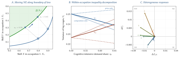
Panel A shows the feasible set \(\mathcal{B}\), with the lower boundary \(\underline{B}(X_1)\) and the contract curve as the cognitive-intensive demand share \(\eta_1\) rises from \(0.50\) to \(0.65\). Asterisks (\(\boldsymbol{*}\)) mark the bundled equilibrium, open circles (\(\circ\)) mark the unconstrained optimum on the contract curve. Panel B shows the within-occupation variance of log wages \(V_j\) for each occupation, decomposed into a price component (dashed, holding composition fixed) and a composition component (dotted, holding prices fixed). Panel C plots the change in cognitive skill price elasticity \(\Delta\beta_{jX}\) against the change in within-occupation inequality \(\Delta V_j\) for \(J=7\) occupations, with points numbered and colored from \(j=1\), the most cognitive-intensive, to \(j=7\), the most manual-intensive. Parameters: independent Fréchet marginals with \(\theta = 2.25\), CES production with \(\sigma = 0.60\), symmetric economy with initial \(\eta_1 = \eta_2 = 0.5\) and \(\overline{X}=\overline{Y}\).
Demand shock: change in wage inequality driven by composition, not prices. Panel B shows the decomposition of the variance of log wages \(V_j\) into price and composition components for each occupation. As in the case of a cognitive-biased technology shock, the demand shock leads to increases in the relative price of cognitive skill, which, on its own, would increase inequality. But where the technology shock led to a same-signed composition effect, albeit a relatively small one, here the demand shock leads to an opposite-signed and large composition effect — large enough to more than overturn the price effect. As occupation 1 expands to meet higher demand, it draws in workers who are less strongly selected on cognitive skill, shifting the mix among its workers away from cognitive skill — the reverse of the technology case — and pushing its wage inequality down. As occupation 2 shrinks, its remaining workers are more strongly selected on manual skill, shifting its mix toward manual skill and pushing its wage inequality up.
Heterogeneous responses across occupations. Panel C shows this for \(J=7\) occupations, reporting how each occupation’s \(V_j\) and cognitive skill price elasticity \(\beta_{jX}\) change as demand shifts toward cognitive-intensive occupations. The demand shift lowers the return to cognitive skill \(\beta_{jX}\) in every occupation because reallocation toward cognitive-intensive occupations shifts the mix of skills away from cognitive skill everywhere: expanding occupations draw in workers less selected on cognitive skill, while contracting occupations shed their most cognitively inclined workers. The most cognitive-intensive occupations are displaced down and to the left, with falling \(\beta_{jX}\) and falling \(V_j\), while the most manual-intensive occupations are displaced up and to the left, with falling \(\beta_{jX}\) but rising \(V_j\).
Can a demand shock explain the trends in within-occupation inequality? From these results we learn a basic lesson: a cognitive-biased demand shock is not a promising explanation of the trends in within-occupation inequality we document in Figure 1. In US data, we see rising inequality in cognitive-intensive occupations, and falling inequality in manual-intensive occupations. But in our model, a demand shock produces the exact opposite pattern. Moreover, as we will see, a demand-based explanation makes two further predictions that are at odds with the data: a demand shock implies a decline in the return to cognitive skill, and large composition changes that co-move positively with occupation-level inequality. Taken together, these facts are a significant challenge to overcome. Indeed, to account for the data a demand-based explanation would have to rely on negative cognitive-biased demand shocks.
5.2.3 Changes in Skill Dispersion
Our final application concerns skill dispersion. In US data we find that workers have become more similar in their measured skills over time, with the within-occupation dispersion in education falling especially sharply in cognitive-intensive occupations. What effect would we expect this to have? To answer this, we reduce the dispersion of cognitive skill \(X\), i.e., increase \(\theta_X\), holding the dispersion of manual skill fixed. As shown in Panel A of Figure 9, a fall in the dispersion of cognitive skill shrinks the feasible set \(\mathcal{B}\) and the equilibrium allocation moves inward to the boundary of the smaller set.
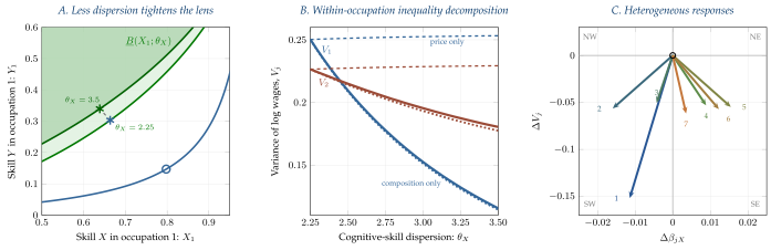
Panel A shows the feasible set \(\mathcal{B}\) as the dispersion of cognitive skill falls, i.e., \(\theta_X\) rises from \(2.25\) to \(3.5\). The feasible set shrinks. Asterisks mark the bundled equilibrium, which moves inward to the boundary of the smaller set (\(\boldsymbol{*}\)); the open circle (\(\circ\)) marks the unconstrained optimum on the contract curve. Panel B shows the within-occupation variance of log wages \(V_j\) for each occupation, decomposed into a price component (dashed, holding composition fixed) and a composition component (dotted, holding prices fixed). Panel C plots the change in cognitive skill price elasticity \(\Delta\beta_{jX}\) against the change in within-occupation inequality \(\Delta V_j\) for \(J=7\) occupations, with points numbered and colored from \(j=1\), the most cognitive-intensive, to \(j=7\), the most manual-intensive. Parameters: independent Fréchet marginals with \(\theta_Y = 2.25\), CES production with \(\sigma = 0.60\), symmetric economy with \(\eta_1 = \eta_2 = 0.5\) and \(\overline{X}=\overline{Y}\).
Panel B shows the decomposition. Almost the entire change in wage dispersion is due to the composition effect. Relative skill prices barely move, so unlike the previous two applications there is essentially no price component to speak of. A fall in the dispersion of cognitive skill compresses wage inequality in both occupations, but far more in the cognitive-intensive occupation 1, whose wages are more exposed to the distribution of cognitive skill. Panel C confirms the same pattern across \(J=7\) occupations. All occupations experience wage compression with the biggest changes in the most cognitively-intensive occupations. The key lesson here is that the substantial rise in wage dispersion we observe in cognitive-intensive occupations is even more striking — it had to overcome a compression in cognitive skill pushing the other way.
Each of these three candidate explanations for changes in within-occupation inequality — technology, demand, and skill dispersion — has a distinct empirical signature, making different predictions about whether prices or composition move a lot or a little and in which direction. A cognitive-biased technology shock raises inequality in cognitive occupations through prices; a demand shift lowers it through composition; and a fall in skill dispersion compresses it. We next measure these effects in US labor market data. Our results suggest the main driver was a cognitive-biased technology shock, whose effect on cognitive occupations was partly offset by a decline in cognitive skill dispersion that pushed the other way. The data are hard to reconcile with a demand-based explanation.
6 Skill Prices and Wage Inequality in US Data
In this section we use US labor market data to show that (i) there are systematic differences in how a given skill is priced across occupations, and (ii) that this variation in skill prices accounts for the bulk of both cross-sectional variation in within-occupation wage inequality and the changes in within-occupation wage inequality from 1980 to 2010. By contrast, we find that selection on observable worker characteristics plays a much more minor role.
We proceed in two steps. First, in Section 6.1, we use the NLSY79, which gives us genuine worker-level measures of cognitive and manual skills, to estimate how these skills are priced across occupations. We find that each skill is valued more highly in occupations which use that skill more intensively, and, crucially, is less valuable in occupations which use the other skill intensively. Second, in Section 6.2, we use the much larger samples of the American Community Survey to estimate how worker-level education and experience are priced across occupations and over time. We find that differences in skill prices account for the bulk of the variation in within-occupation inequality across occupations and of its rise from 1980 to 2010, with the rise concentrated in cognitively-intensive occupations, where the return to education rose most steeply.
6.1 Skills Are Priced Differently Across Occupations
NLSY79. We begin with the National Longitudinal Survey of Youth 1979, which follows a cohort of Americans from their late teens and early twenties through their working lives. Importantly for our purposes, the NLSY79 provides direct measures of workers’ cognitive and manual skills, through aptitude tests administered before or near labor market entry. With these measures we can ask whether the same skill commands a different price in different occupations. We observe each worker’s occupation at a detailed three-digit level. But, because in many three-digit occupations there are too few NLSY79 workers to estimate skill prices precisely, we aggregate occupations into two-digit occupation groups, estimating prices within each group while retaining the detailed occupations as controls. This gives us enough workers per group to price skills reliably and enough groups to compare those prices across occupations. We use all survey waves. After cleaning the data we are left with roughly 128,000 person-year observations on some 9,600 workers. We provide the full details of our dataset and sample construction in Appendix A.
Group-level Mincer regression. Following the log wage equation (18), we estimate how skills are priced from a worker-level regression of log hourly wages on measured skills and controls, run separately within each group \(g\) \[\tag{46} \ln w_{it} \;=\; \alpha_{j(it)} \;+\; \boldsymbol{x}_{i}'\boldsymbol{\beta}_{g} \;+\; \boldsymbol{X}_{it}'\boldsymbol{\delta}_{g} \;+\; \varepsilon_{it},\qquad i\in g\] where \(i\) indexes workers, \(t\) indexes survey years, and \(\boldsymbol{x}_{i} = (\mathrm{cog}_i,\,\mathrm{man}_i,\,\mathrm{edu}_i)'\) collects a worker’s time-invariant cognitive skill, manual skill, and years of schooling. Because the regression is run separately for each group, all coefficients are group-specific. Our interest is in the skill prices \(\boldsymbol{\beta}_{g} = (\beta_g^{\mathrm{cog}},\,\beta_g^{\mathrm{man}},\,\beta_g^{\mathrm{edu}})'\). The remaining controls \(\boldsymbol{X}_{it}\) are experience and its square, sex, race, log hours, and a quadratic year trend. The fixed effect \(\alpha_{j(it)}\) is for the detailed occupation \(j(it)\) in which worker \(i\) is employed at \(t\), nested within group \(g\), so the skill prices \(\boldsymbol{\beta}_g\) are identified entirely from variation within detailed occupations, not from differences across occupations in average wages and average skills. We estimate (46) for each of the \(G=63\) two-digit groups with at least \(100\) person-years and at least three distinct detailed occupations, pooling the NLSY79 panel across survey years.7
Skill prices and task intensities. For each occupation group \(g\), the regression (46) gives us an estimated price of cognitive skill \(\beta_g^{\mathrm{cog}}\) and of manual skill \(\beta_g^{\mathrm{man}}\). Our framework predicts that, in a bundled equilibrium, these prices both vary across occupations and vary directly with how intensively each occupation uses each skill. To measure skill intensity we use standard Autor and Dorn (2013) estimates of the cognitive and manual task content of each occupation, taken from O*NET, and averaged within groups. We then ask how each skill price varies across groups with each task intensity. For a skill \(k\in\{\mathrm{cog},\mathrm{man}\}\) and a task intensity \(\tau\in\{\mathrm{cog},\mathrm{man}\}\), the across-group gradient \(\gamma_{\tau}^{k}\) is the \(\sqrt{N_g}\)-weighted8 slope of the skill price \(\beta_g^{k}\) on the task intensity \(\tau_g\) \[\tag{47} \gamma_{\tau}^{k} \;=\; \frac{\sum_g \sqrt{N_g}\,\big(\tau_g-\bar\tau\big)\big(\beta_g^{k}-\bar\beta^{k}\big)}{\sum_g \sqrt{N_g}\,\big(\tau_g-\bar\tau\big)^2}\] where \(\bar\tau\) and \(\bar\beta^{k}\) are the corresponding weighted means across groups. The two skills and two intensities give four gradients. Figure 10 plots our estimates of these gradients. The diagonals relate each skill’s price to the intensity of the same skill (\(\gamma_{\mathrm{cog}}^{\mathrm{cog}}\) and \(\gamma_{\mathrm{man}}^{\mathrm{man}}\)). The off-diagonals relate each skill’s price to the intensity of the other skill (\(\gamma_{\mathrm{man}}^{\mathrm{cog}}\) and \(\gamma_{\mathrm{cog}}^{\mathrm{man}}\)).
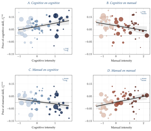
Each point is an occupation group \(g\). The vertical axis is the estimated price of cognitive skill, \(\beta_g^{\rm cog}\) (top row), or of manual skill, \(\beta_g^{\rm man}\) (bottom row), estimated from the worker-level regression (46) with controls for education, experience, sex, race, hours, and fixed effects for each detailed three-digit occupation within group \(g\). Cognitive and manual skill are measured by the worker’s AFQT score and a manual ASVAB composite respectively. The horizontal axis is the group’s mean cognitive (left column) or manual (right column) task intensity, standardized across groups. Marker area is proportional to the number of person-years in group \(g\), and marker color indicates terciles of the task intensity on the horizontal axis. The solid line is the weighted least-squares fit of the gradient (47). The shaded region is the pointwise 95% confidence band for the fit. The gradient and its bootstrap standard error for each panel are reported in Table 2. NLSY79, 1980–2022; \(G=63\) two-digit occupation groups; 128,246 person-year observations.
Positive diagonals: prices of primary skills vary across occupations. The two diagonal panels of Figure 10 show that each skill is priced more highly in occupations that use it more intensively. The price of cognitive skill rises with cognitive task intensity, \(\gamma_{\rm cog}^{\rm cog} = +0.027\) (Panel A), and the price of manual skill rises with manual task intensity, \(\gamma_{\rm man}^{\rm man} = +0.023\) (Panel D). Both gradients are positive and statistically significant, as shown in Table 2. Because skill is measured in standard deviations and task intensity is standardized across groups, these magnitudes are economically large. Moving to an occupation one standard deviation higher in cognitive task intensity raises the return to a standard deviation of cognitive skill by \(0.027\) log points, or approximately \(2.7\%\) — roughly one-third of its cross-occupation average return of \(7.7\%\). Across the full range of occupations, from the least to the most cognitively intensive, the return to cognitive skill roughly doubles. These positive own-intensity gradients are the pattern predicted by a bundled equilibrium in the Example of Section 4.2.2 and are evidence against an unbundled equilibrium. If the law of one price for skills holds, a unit of cognitive skill would command the same price in all occupations and the gradient would be zero. The data clearly reject this.
| Gradient \(\gamma_{\tau}^k\) | Average \(\bar{\beta}^k\) | ||
|---|---|---|---|
| Cognitive task intensity | Manual task intensity | ||
| Cognitive skill price | \(+0.027\) | \(-0.018\) | \(+0.077\) |
| \((0.007)\) | \((0.006)\) | \((0.006)\) | |
| Manual skill price | \(-0.019\) | \(+0.023\) | \(+0.005\) |
| \((0.008)\) | \((0.007)\) | \((0.007)\) | |
The first two columns report the cross-occupation gradients \(\gamma_\tau^k\) from (47), the weighted slope across two-digit occupation groups of the within-occupation price of skill \(k\) on Autor and Dorn (2013) task intensity \(\tau\). The final column, \(\bar\beta^k\), is the weighted average price of skill \(k\) across groups. Standard errors in parentheses are from a block bootstrap with \(500\) resamples. NLSY79, 1980–2022.
Negative off-diagonals: prices of secondary skills vary across occupations. The two off-diagonal panels of Figure 10 show that each skill is priced less highly in occupations that use the other skill more intensively. The price of cognitive skill falls with manual task intensity, \(\gamma_{\rm man}^{\rm cog} = -0.018\) (Panel B), and the price of manual skill falls with cognitive task intensity, \(\gamma_{\rm cog}^{\rm man} = -0.019\) (Panel C). These gradients are negative and statistically significant, under bootstrap and classical standard errors alike.9 These effects are sizable: a one-standard-deviation increase in manual intensity lowers the cognitive price by \(0.018\) log points, about two-thirds the size of the own-intensity diagonal. How intensively an occupation uses the secondary skill matters nearly as much as how intensively it uses the primary skill. Together with the positive diagonals, these negative off-diagonals complete the full set of \(2\times2\) effects predicted by the Example of Section 4.2.2. In an unbundled equilibrium, all of these gradients would be zero.
Differences in average skill prices. A notable feature of these estimates is how differently the two skills are priced on average. Averaged across occupations, the return to an additional standardized unit of cognitive skill within an occupation is substantial, \(+0.077\), while the price of a standardized unit of manual skill is \(+0.005\) and, with a bootstrap standard error of \(0.007\), statistically indistinguishable from zero. Within occupations, cognitive skill is highly valued in the labor market and more so in cognitively intensive occupations. Because cognitive skill is both more valuable on average within an occupation and this return increases across occupations, it matters much more for wage inequality.
Overall, these results establish that skill prices vary across occupations, and in a way that is consistent with a bundled equilibrium in our model. But because the NLSY79 has modest samples and a single cohort whose aging is confounded with calendar time, it cannot tell us how much of within-occupation wage inequality is accounted for by skill prices and how, if at all, changes in skill prices have contributed to changes in wage inequality over time. For this we need the much larger samples of the American Community Survey, to which we now turn.
6.2 Skill Price Differences Explain Within-Occupation Wage Inequality
ACS. The American Community Survey is large enough that we can estimate skill prices for each three-digit occupation directly, through repeated cross-sections over time, each a fresh sample of all ages rather than a single aging cohort. But the ACS lacks direct measures of worker-level skills. We know a worker’s education and labor market history but do not have the aptitude tests available in the NLSY. Because of this, we price worker-level education and experience, with education standing in for the cognitive skill that the NLSY measured directly. As before, we estimate skill prices occupation by occupation, now allowing them to vary across three-digit occupations \(j\) and over years \(t\).
Occupation-level Mincer regression. For each occupation \(j\) and year \(t\) we estimate skill prices from the analogue of (46), now run separately for each occupation in each year, \[\tag{48} \ln w_{i} \;=\; \alpha_{jt} \;+\; \boldsymbol{x}_{i}'\boldsymbol{\beta}_{jt} \;+\; \boldsymbol{X}_{i}'\boldsymbol{\delta}_{jt} \;+\; \varepsilon_{i},\qquad i\in (j,t)\] where \(\alpha_{jt}\) is an occupation-year intercept, and \(\boldsymbol{x}_{i} = (\mathrm{edu}_{i},\,\exp_{i},\,\exp_{i}^2)'\) collects a worker’s years of schooling and experience. Our interest is again the skill prices \(\boldsymbol{\beta}_{jt}\). The remaining controls \(\boldsymbol{X}_{i}\) are sex, race, and log hours, the same as applied in Table 1 and Figure 1. We estimate (48) on Census 1980 and ACS 2010 samples for each occupation with at least \(100\) workers, giving \(J=286\) occupations observed in both 1980 and 2010. The samples are very large — roughly three million workers in 1980 and nearly one million in 2010, against some 9,600 workers in the NLSY79. Full details of our Census and ACS samples are provided in Appendix A.
With the skill prices in hand, we proceed in three steps. First, we show that differences in skill prices account for almost all of the variation in within-occupation wage inequality across occupations, while differences in the distribution of skills across workers account for little. Second, we show that changes in skill prices, rather than changes in the distribution of skills, account for most of the rise in within-occupation inequality from 1980 to 2010. Third, we show that the aggregate rise in within-occupation inequality is concentrated in cognitively intensive occupations. About three-fifths of employment is in occupations where both the price of education and within-occupation inequality rose, and the top two terciles of cognitively intensive occupations account for around \(90\%\) of the rise.
6.2.1 Skill Price Differences Across Occupations
Within-occupation wage inequality. Our object of interest is within-occupation wage inequality. From the regression (48), the portion of this inequality attributable to differences in priced skills among workers is the within-occupation variance of fitted log wages \[\tag{49} V_{jt} \;:=\; \mathrm{Var}_{j}\!\left[\boldsymbol{x}_{i}'\boldsymbol{\beta}_{jt}\right] \;=\; \boldsymbol{\beta}_{jt}'\,\boldsymbol{\Sigma}_{jt}\,\boldsymbol{\beta}_{jt}\] where \(\boldsymbol{\Sigma}_{jt}\) is the covariance matrix of the observed skills \(\boldsymbol{x}_{i}\) among workers in occupation \(j\) in year \(t\). For brevity we refer to \(V_{jt}\) as the within-occupation variance, with the understanding that it is the variance attributable to the priced skills \(\boldsymbol{x}_i\). The variance \(V_{jt}\) is determined by two components: (i) the skill prices \(\boldsymbol{\beta}_{jt}\), which tell us how each skill is rewarded, and (ii) the skill dispersion \(\boldsymbol{\Sigma}_{jt}\), which tells us how skills are distributed in that occupation. Within-occupation inequality is high when skills are highly priced and widely dispersed.
Skill prices and cognitive intensity. To understand how this relates to our NLSY results, Panel A of Figure 11 reports how the price of education \(\beta_{j}^{\rm edu}\) in 2010 varies with cognitive intensity. This is the same gradient concept that we calculated for the NLSY, now applied to education. The price of education varies across occupations and is systematically higher in more cognitively intensive occupations, with a gradient of \(+0.015\). Averaged across occupations, a year of schooling raises wages by about \(6\%\), a familiar Mincerian return. But this average masks wide variation. The price of education rises from under \(2\%\) per year of schooling in the least cognitively intensive occupations to nearly \(10\%\) in the most.
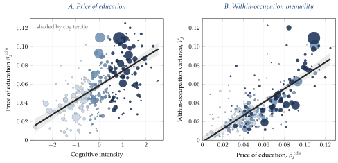
Each point is a three-digit occupation \(j\). Panel A plots the within-occupation price of education \(\beta_{j}^{\rm edu}\) against the occupation’s Autor and Dorn (2013) measure of cognitive task intensity. The weighted fit has gradient \(+0.015\). Panel B plots within-occupation variance \(V_j\) against the price of education \(\beta_{j}^{\rm edu}\). The weighted fit has gradient \(+0.710\). The within-occupation variance \(V_j = \boldsymbol{\beta}_j'\boldsymbol{\Sigma}_j\boldsymbol{\beta}_j\) where \(\boldsymbol{\Sigma}_{j}\) is the covariance matrix of the observed skills \(\boldsymbol{x}_{i}=(\mathrm{edu}_{i},\,\exp_{i},\,\exp_{i}^2)\) among workers in occupation \(j\). The Mincer regression (48) also controls for sex, race, and log hours with occupation-specific coefficients. Marker area is proportional to occupation sample size and marker color indicates terciles of cognitive task intensity. The shaded regions are pointwise \(95\%\) confidence bands. For visual clarity the panels are clipped to the employment-weighted 1st–99th percentile of the plotted variables. The four observations outside the frame in Panel A are those with negative estimated education prices, accounting for 0.2% of employment; a further 1.2% of employment lies outside the frame in Panel B. All of these outliers are retained in all estimation. ACS 2010 cross-section, \(J = 287\) occupations.
In this sense the ACS reproduces our NLSY finding, now estimated far more precisely and across hundreds of detailed occupations. Moreover Panel B of Figure 11 shows that within-occupation inequality \(V_{jt}\) rises steeply with the price of education \(\beta_{jt}^{\rm edu}\). Occupations that pay more for a year of schooling have substantially more dispersed wages. Taken together, the two panels show that within-occupation inequality is highest in exactly those cognitively intensive occupations where education is most highly priced. But is it differences in skill prices \(\boldsymbol{\beta}_{jt}\) across occupations that generate this pattern, or differences in the dispersion of skills \(\boldsymbol{\Sigma}_{jt}\) among their workers?
A dual decomposition. To decompose within-occupation wage inequality \(V_{jt}\) into its skill-price and skill-composition components, we construct counterfactual variances that hold one component at its cross-occupation average while letting the other vary. Let \(\bar{\boldsymbol{\beta}}_t = \sum_j s_{jt}\,\boldsymbol{\beta}_{jt}\) and \(\bar{\boldsymbol{\Sigma}}_t = \sum_j s_{jt}\,\boldsymbol{\Sigma}_{jt}\) denote the employment-weighted average price vector and skill dispersion across occupations in year \(t\). We then define price-only and composition-only counterfactual variances \[\tag{50} V_{jt}^{\boldsymbol{\beta}} \;=\; \boldsymbol{\beta}_{jt}'\,\bar{\boldsymbol{\Sigma}}_t\,\boldsymbol{\beta}_{jt}, \qquad\qquad V_{jt}^{\boldsymbol{\Sigma}} \;=\; \bar{\boldsymbol{\beta}}_t'\,\boldsymbol{\Sigma}_{jt}\,\bar{\boldsymbol{\beta}}_t\] The price-only variance \(V_{jt}^{\boldsymbol{\beta}}\) tells us what within-occupation inequality would be if occupation \(j\) had its own skill prices but the economy-wide average skill composition. The composition-only variance \(V_{jt}^{\boldsymbol{\Sigma}}\) does the reverse, telling us what inequality would be if occupation \(j\) had its own skill composition but the economy-wide average skill prices. We can then write \(V_{jt} = V_{jt}^{\boldsymbol{\beta}} + V_{jt}^{\boldsymbol{\Sigma}} + V_{jt}^{\rm int}\) where the interactions are summarized by a residual that ensures the components sum to \(V_{jt}\). To determine which component is responsible for the cross-occupation pattern in Figure 11, we compare the gradient of each counterfactual variance with respect to cognitive intensity. If one of these counterfactual variances has the same gradient as the actual variance \(V_{jt}\), then that component is responsible for most of what we see in the data.
Prices account for the cross-occupation gradient. The results from the decomposition are stark, as shown in Figure 12. Prices account for almost all of the cross-occupation gradient. Panel A reports for 2010 the price-only counterfactual variance \(V_{jt}^{\boldsymbol{\beta}}\) against cognitive intensity alongside the actual variance \(V_{jt}\). The two are nearly indistinguishable, rising together at almost exactly the same rate. Panel B plots the composition-only counterfactual variance \(V_{jt}^{\boldsymbol{\Sigma}}\), which is essentially flat. Differences in skill prices across occupations account for \(98\%\) of the cross-occupation gradient in within-occupation inequality, basically all of it, while differences in the composition of observed skills account for basically none of it. The cross-occupation pattern in within-occupation inequality is, to a first approximation, entirely a matter of how skills are priced. As we show in Appendix B.2, prices dominate in 1980 as well, though less starkly.
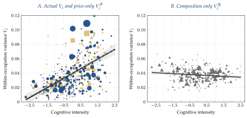
Each point is a three-digit occupation \(j\), plotted against the occupation’s Autor and Dorn (2013) measure of cognitive task intensity. Panel A compares the actual within-occupation variance \(V_{j}\) (blue circles) with the price-only counterfactual \(V_{j}^{\boldsymbol{\beta}}=\boldsymbol{\beta}_{j}'\,\bar{\boldsymbol{\Sigma}}\,\boldsymbol{\beta}_{j}\) (gold squares), which gives each occupation its own vector of skill prices \(\boldsymbol{\beta}_{j}\) but the economy-wide employment-weighted average skill composition \(\bar{\boldsymbol{\Sigma}}\). The two have essentially identical gradients (\(+0.013\)). The actual variance is drawn with a solid line and the price-only counterfactual with a dashed line. Panel B plots the composition-only counterfactual \(V_{j}^{\boldsymbol{\Sigma}} = \bar{\boldsymbol{\beta}}'\,\boldsymbol{\Sigma}_{j}\,\bar{\boldsymbol{\beta}}\) (grey triangles), which gives each occupation its own skill composition \(\boldsymbol{\Sigma}_{j}\) but the economy-wide employment-weighted average vector of skill prices \(\bar{\boldsymbol{\beta}}\). Its gradient is essentially flat (\(-0.001\)). Marker areas are proportional to occupation sample size. For visual clarity the panels are clipped to the employment-weighted 1st–99th percentile of the plotted variables. All outliers are retained in all estimation. ACS 2010 cross-section, \(J = 287\) occupations.
6.2.2 Changes in Skill Prices over Time
Within-occupation wage inequality not only differs across occupations but has also risen substantially over recent decades. From 1980 to 2010 the average within-occupation variance \(V_{jt}\) rose from 0.030 to 0.041, by more than a third. We have shown that prices explain almost all of the differences in \(V_{jt}\) across occupations. Do changes over time also reflect changes in skill prices, or changes in the composition of workers within occupations?
A decomposition over time. For each occupation \(j\) we calculate the change in the within-occupation variance from 1980 to 2010, \(\Delta V_{j} = V_{j,2010} - V_{j,1980}\). We then split this into a price channel \(\Delta V_{j}^{\boldsymbol{\beta}}\), which holds each occupation’s skill composition at its 1980 level and lets only its prices change to 2010. The composition channel \(\Delta V_{j}^{\boldsymbol{\Sigma}}\) does the reverse, holding prices at their 1980 level and letting only composition change. As in the cross-section, an interaction term accounts for the small remainder, so that \(\Delta V_{j} = \Delta V_{j}^{\boldsymbol{\beta}} + \Delta V_{j}^{\boldsymbol{\Sigma}} + \Delta V_{j}^{\rm int}\). We then aggregate across occupations, weighting each by its 1980 share of employment.
Prices drive the rise in inequality. Changes in skill prices drive the rise in \(V_{jt}\). In fact, had prices changed as they did but the composition of workers stayed fixed at its 1980 level, within-occupation inequality would have risen by even more than it actually did. Aggregated across occupations, we find \(\Delta V^{\boldsymbol{\beta}} = +0.014\) whereas the actual rise was \(\Delta V = +0.011\). Far from driving the rise, the change in composition softened it, \(\Delta V^{\boldsymbol{\Sigma}} = -0.001\). This softening reflects in large part a reduction in the dispersion of education within occupations. Over this period, the within-occupation variance of schooling fell from 5.4 to 4.9 on average. And this fall was concentrated in the most cognitively intensive occupations, which in 1980 had the most dispersed schooling of all, at 6.2, but by 2010 had fallen back to the average, 4.9, a fall of more than 20%. How much of the overall rise in residual within-occupation wage inequality does this account for? From Table 1, residual within-occupation wage inequality increased by \(+0.031\) from 1980 to 2010, so a share of about \(0.011/0.031\approx0.36\) of the rise in residual wage inequality is accounted for by changes in the variance attributed to priced skills \(V_{jt}\). Since the change in \(V_{jt}\) is itself overwhelmingly due to changes in skill prices, overall we find that changes in skill prices account for about a third of the aggregate rise in within-occupation wage inequality.
The price of education steepened. Why did within-occupation inequality rise by so much in some occupations while rising modestly or falling in others? The key is that the price of education did not rise uniformly across occupations. It rose most in the occupations that were already most cognitively intensive. The cross-occupation gradient of the education price on cognitive intensity steepened from \(\gamma_{1980} = +0.009\) in 1980 to \(\gamma_{2010} = +0.015\) in 2010. Regressing the change in each occupation’s education price on its cognitive intensity confirms this, with a gradient of \(\gamma_{\Delta} = +0.006\).10 Figure 13 shows the underlying trajectories. Each arrow is the trajectory of an occupation’s price of education \(\beta_{j}^{\rm edu}\) and its within-occupation variance \(V_{j}\) from its 1980 position to its 2010 position. Occupations with statistically significant changes in the price of education \(\beta_{j}^{\rm edu}\) from 1980 to 2010 are colored. The remaining occupations are shown as fine light grey arrows. About 75% of the employment in the top cognitive tercile is in occupations that moved in the northeast direction, up and to the right, with the price of education and within-occupation inequality both increasing. Pooled across all occupations, moves up and to the right account for about three-fifths of all employment.
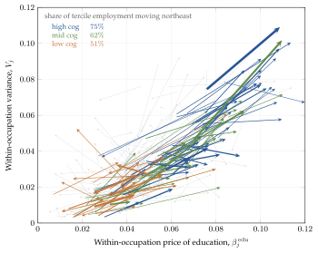
Each arrow is the trajectory of an occupation’s price of education \(\beta_{j}^{\rm edu}\) and its within-occupation variance \(V_{j}\) from its 1980 position to its 2010 position. Occupations with statistically significant changes in the price of education \(\beta_{j}^{\rm edu}\) from 1980 to 2010 are colored. The remaining occupations are shown as fine light grey arrows. The arrows are colored by tercile of cognitive intensity (low, orange; middle, green; high, blue), and arrow width is proportional to 1980 occupation employment. The inset reports the share of each tercile’s employment that moved to the northeast, with both the education price and within-occupation variance rising. Pooled across all occupations, changes in the northeast (NE) direction with both rising skill price and rising inequality account for \(62\%\) of employment. Changes in the southwest, northwest and southeast directions account for 13%, 16% and 9% of employment respectively. For visual clarity the axes are clipped to the employment-weighted 1st–99th percentile of the plotted variables. About 1.7% of employment lies outside this frame but is retained in all calculations. Census 1980 and ACS 2010, \(J = 286\) occupations observed in both years.
6.2.3 The Aggregate Rise in Within-Occupation Inequality
To this point we have considered each occupation and asked what drove the changes in its wage inequality. The answer is, basically, changes in skill prices. We now take a step back and ask which occupations are most responsible for the aggregate rise. The answer is, basically, the cognitively intensive occupations. This conclusion is driven by three interconnected results:
The rise is within occupations, not across them. Aggregate within-occupation inequality could rise either because occupations become more internally unequal or because employment shifts toward occupations that are already unequal. But a shift-share decomposition, reported in Appendix B.4, shows that the first of these dominates. Most of the rise reflects occupations becoming more unequal internally, not the reallocation of workers toward unequal occupations.11
The rise is concentrated in cognitively intensive occupations. The occupations that became more unequal are overwhelmingly those in which the price of education also rose, the occupations climbing toward the upper-right of Figure 13, and these are overwhelmingly the cognitively intensive ones. Where the price of education rose, inequality rose, and both rose most where cognitive skill is most intensively used.12
This is what our framework predicts. When the productivity of cognitive skill rises uniformly across the economy, the bundling friction makes the price of cognitive skill rise by more in more cognitively intensive occupations. Within-occupation inequality therefore rises by more in cognitively intensive occupations and by less in manually intensive ones.
All told, it is not who the workers are, but what their skills are worth, that drives the rise in inequality. In the data, workers have become more alike in their education, especially in cognitive occupations, which have gone from being outliers on the high side to having average levels of education dispersion. By itself, this compression would have reduced within-occupation inequality, and it poses something of a challenge for models in which within-occupation inequality is driven by skill dispersion. But we find that the rising market value of skills, particularly cognitive skills, more than offset the compression in skill dispersion and drove the aggregate rise in within-occupation inequality.
7 Conclusion
We find that, to a first approximation, within-occupation wage inequality is a matter of how skills are priced rather than of who works where. Both cognitive and manual skills are priced differently across occupations. These differences in skill prices explain why within-occupation inequality is higher in more cognitively intensive occupations. They also account for ‘more than all’ of the rise in within-occupation inequality associated with observable skills, and about a third (36%) of the overall rise, from 1980 to 2010. By contrast, differences in the composition of workers play a minor role. Over this period, workers within occupations became more alike in their skills, especially in the cognitively intensive occupations where inequality rose most. The rising market return to cognitive skill was sharp enough to overwhelm this compression, driving inequality up even in occupations where skill dispersion was falling.
Our analysis assumes competitive labor markets, with each worker paid the market price for their skills in their chosen occupation. This competitive setting permits a sharp characterization of how skill supply, skill demand, and the bundling friction interact to jointly determine both equilibrium skill prices and the composition of workers in each occupation. We also focus on the variation in wages attributable to observable skills being paid differently in different occupations. Other labor market frictions, including search frictions, provide a complementary theory of pure residual wage dispersion — why observationally equivalent workers may be paid differently, as in Burdett and Mortensen (1998). An important recent strand of this literature, including Lise and Postel-Vinay (2020) and Lindenlaub and Postel-Vinay (2023), shares with us an emphasis on sorting when workers and jobs have multiple attributes. A key challenge for future research is to construct equilibrium models that incorporate bundling and search-and-matching frictions, so as to jointly determine equilibrium skill prices and worker mobility within and across occupations.
The labor market outcomes in our framework are efficient and there is no role for welfare-improving policy interventions. A large literature, following Manning (2003), argues that employers possess substantial wage-setting power, so that observed wages are marked down below marginal products. A recent strand of this literature, including Lamadon et al. (2022) and Berger et al. (2022), structurally estimates the extent of labor market power and evaluates labor market policies in this context. A natural direction for future research would be to embed the bundling friction in structural models of this kind, allowing policies that tax or subsidize skill supply or demand to be evaluated in terms of their effects on employment, wages, and welfare.
Our analysis takes technology and labor supply as given. In an earlier version of this paper we allowed firms to choose optimal skill intensities from a menu of technologies, as in Caselli and Coleman (2006), so that the equilibrium technology is itself determined jointly with skill prices. We showed that an active technology choice can change the bundling outcome. When skills are substitutes in production, firms adopt technologies that tighten the bundling constraint, so that an initially unbundled equilibrium can become endogenously bundled, raising skill premia and within-occupation inequality; when skills are complements, the reverse occurs, and an initially bundled equilibrium can become endogenously unbundled. This extension provides a natural framework for understanding how the introduction of new technologies can reshape the market returns to skill. Another natural extension is to allow for elastic labor supply, on either the intensive margin (hours) or extensive margin (participation). Both tend to relax the bundling friction, since, other things equal, they make it easier for the economy to deliver the allocation of skills demanded by occupation-level technologies. Elastic labor supply allows the model to speak to inequality in hours and earnings, not just wages. The bundling friction also introduces a distinctive consideration on the extensive margin: because a worker’s participation decision depends on their wage in their best occupation, the bundling friction is particularly important for workers with a strong comparative advantage.
While these extensions are natural directions for future research, our analysis in this paper is deliberately focused on a single fundamental mechanism. Changes in technology that increase the demand for a skill raise its price everywhere, but most of all in the occupations that use the skill most intensively. This uneven incidence generates changes in inequality both within and across occupations, leading to sharply higher pay for the workers who have a lot of a skill in an occupation that finds it increasingly valuable.
References
A Data
In Appendix A.1 we explain how we use the 5% state sample of the 1980 decennial Census and the 1% one-year sample of the 2010 American Community Survey (ACS), both available as part of the Integrated Public Use Microdata Series (IPUMS) — see Ruggles et al. (2025) for details. In Appendix A.2 we explain how we use data from the National Longitudinal Survey of Youth 1979 (NLSY79).
A.1 Census and ACS Samples
Basic sample restrictions. We restrict our
1980 Census and 2010 ACS samples to working-age workers attached to the
labor market on a full-time, year round basis. Specifically, we restrict
to workers aged between 18 and 64 during the earnings year with positive
person weight (perwt) who worked at least 48 weeks in the
previous year (wkswork1, or the wkswork2
bracket midpoint where it is not reported) and at least 30 usual weekly
hours (uhrswork) with wage and salary income
(incwage) of at least $1,000. We also drop residents of
institutional group quarters (gqtyped 100–499) and unpaid
family workers (classwkrd 29) and drop occupation codes for
military and unclassified workers. These restrictions leave us with
2,973,801 observations in 1980 and 935,966 observations in 2010.
Two features of this sample are worth further comment. First, the $1,000 earnings floor is nominal and applies equally in both 1980 and 2010. The real-equivalent floor in 2010 is about $3,000. We have experimented with imposing that higher floor. It excludes about 480 workers from our 2010 sample whose implied wages are implausibly low, with a median of $0.78 per hour. Excluding these workers changes the total, within and residual variance of log wages in 2010 from 0.407/0.286/0.270 in Table 1 to 0.405/0.285/0.269. Second, the sample is not restricted to wage and salary workers. Self-employed workers with positive wage and salary income are retained, and constitute 3.8% of employment in 1980 and 4.2% in 2010. Indeed, two-thirds of the 480 workers admitted by the nominal earnings floor in 2010 are self-employed, many of them farmers. Appendix B.7 reports our main variance decomposition under alternative treatments of self-employed workers.
Weeks worked. We measure weeks worked in the 1980 Census directly. The 2010 ACS reports weeks worked in brackets, and every 2010 observation is assigned its bracket midpoint. In practice this is a single value — 98% of the 2010 sample falls in one bracket and is assigned 51 weeks, against a mean of 51.6 weeks actually reported in 1980. Using the 1980 distribution of weeks as a reference, this 2010 interval measure adds a log variance of about 0.0004, roughly one percent of the measured change in within-occupation inequality.
Wages. We measure the hourly wage as
annual wage and salary income (incwage) divided by the
product of usual weekly hours (uhrswork) and weeks worked
in the previous year. Log hourly wages are winsorized at the
perwt-weighted 1st and 99th percentiles within
occ1990 occupation cells, separately by year. This is done
before the occupation crosswalk discussed below and before any cell-size
selection.
Occupations. We harmonize
occ1990 3-digit occupation codes to occ1990dd
codes using the crosswalk provided by David Dorn. The crosswalk fails to
match one occupation code, accounting for 489 observations in 1980 and
76 in 2010, under 0.02% of the sample in either year. We retain
occupations with at least 100 observations, leaving 326 occupations in
1980 and 291 in 2010, with 290 present in both years. Four occupations
in each year lack a task intensity score, as discussed below, and one
further 1980 occupation falls below the threshold once the regression
sample is formed. This leaves 322 occupations in the 1980 cross-section,
287 in the 2010 cross-section, and \(J=286\) occupations present in both
years.
Task intensities. We measure an occupation’s cognitive and manual task intensities using the time-invariant scores provided by Autor and Dorn (2013). These scores are standardized on the \(J=286\) occupations present in both years for which we have valid task intensity scores. The same location and scale are then applied to each year’s cross-section, so that task intensity is in common units across all exhibits. Task intensity terciles are the unweighted thirds of the standardized index on the same 286 occupations.
Education. We measure education as years
of schooling from the IPUMS code educ, which reports
completed schooling in categories. From 1990 on the Census and ACS have
classified high school graduates by highest degree attained rather than
by highest year completed, and educ harmonizes the two
schemes by assigning each degree the number of years it typically takes.
One consequence of this is that there is a category for three years of
college in 1980 with no exact equivalent in 2010, so years of schooling
are constructed from a slightly coarser partition in the later year. To
assess how much this matters we recompute the within-occupation variance
of schooling with the some college categories
collapsed to a common value in both years. For our benchmark calculation
the fall in the variance is 0.521, from 5.405 to 4.884, while under the
harmonized partition the fall is 0.479.
Weights. We average across observations
using the IPUMS person weight perwt. In the 1980 Census
this weight is uniform, while in the 2010 ACS this weight varies, with a
coefficient of variation of about 0.10. We aggregate across occupations
using 1980 employment shares constructed using person weights —
equivalently, 1980 occupation sample sizes. Cross-occupation regressions
are weighted by the square root of occupation cell size, and figures
scale marker area by occupation cell size.
A.2 NLSY79 Sample
Basic sample restrictions. We restrict our NLSY79 sample to respondents aged 23 and over who are not currently enrolled in school and who report an hourly wage, an occupation, an AFQT score, completed schooling and hours worked. We drop the military oversamples. These restrictions leave us with 128,246 person-years for 9,620 respondents, observed between 1980 and 2022.
Wages. We measure the hourly wage as the respondent’s reported rate of pay on their main job. Wages are trimmed to the range $1 to $200. As with the Census and ACS earnings floor, these bounds are nominal and apply equally across all survey years. Hours are measured as hours worked in the past calendar year divided by weeks worked in the past calendar year, giving usual hours per week.
Occupations. Occupation is coded in three
Census vintages over the survey period. We take the 1980 code where it
is available, then the 2000 code, then the 1970 code, and harmonize each
to occ1990dd using the corresponding crosswalk. This
succeeds for 99.3% of person-years. Because a detailed occupation holds
too few person-years to estimate a skill price, we pool to two-digit
groups. We retain groups with at least 100 person-years and at least
three detailed occupations, leaving \(G=63\) groups from 83 candidates. The
median group holds 1,034 person-years and five detailed occupations.
Skills. We measure cognitive skill by the 1989-revised AFQT score and manual skill by the sum of the three mechanical ASVAB section scores — Auto and Shop Information, Mechanical Comprehension, and Electronics Information — which are distinct from the four subtests underlying AFQT. Both measures are standardized on the analytic sample. Across respondents the correlation between the two skill measures is 0.74.
Task intensities. A group’s task intensity is the person-year weighted mean of the task intensities of its detailed occupations, using the same Autor and Dorn (2013) scores as in the Census and ACS samples.
B Additional Empirical Results
In this appendix we report additional details of our empirical results and related robustness checks referred to in the main text.
B.1 Within-Occupation Inequality by Occupational Group
Table B.1 reports residual within-occupation wage inequality in 1980 and 2010 for 16 broad occupational groups. For each group we average over individual occupations using fixed 1980 employment weights. From 1980 to 2010, within-occupation wage inequality increased in most groups, 11 out of 16, accounting for more than 80% of employment. Consistent with our findings in Section 6.2.2, the increases are concentrated in more cognitively-intensive occupation groups, including Sales (\(+0.106\)), Managers and Administrators (\(+0.090\)), and Engineers and Scientists (\(+0.056\)). The decreases are concentrated in more manually-intensive occupation groups, including Construction and Mining (\(-0.007\)), Material Moving and Laborers (\(-0.019\)), and Transportation (\(-0.034\)). Farming, Forestry and Fishing (\(-0.125\)) is an important outlier, a much larger decrease than any other group. The group is relatively small, accounting for about 1.2% of employment in 1980. The large decrease here reflects changes in the measurement of farm earnings, as discussed in more detail in Appendix B.7 below.
| Residual within-occ. variance | Employment share | ||||
|---|---|---|---|---|---|
| 1980 | 2010 | Change | 1980 | 2010 | |
| Groups with rising within-occupation inequality | |||||
| Sales | 0.331 | 0.437 | 0.106 | 0.088 | 0.102 |
| Managers and Administrators | 0.291 | 0.381 | 0.090 | 0.138 | 0.160 |
| Engineers and Scientists | 0.151 | 0.206 | 0.056 | 0.031 | 0.042 |
| Clerical and Admin. Support | 0.155 | 0.196 | 0.041 | 0.189 | 0.151 |
| Protective Service | 0.203 | 0.238 | 0.036 | 0.019 | 0.026 |
| Technicians | 0.183 | 0.214 | 0.032 | 0.034 | 0.043 |
| Machine Operators and Assemblers | 0.213 | 0.224 | 0.011 | 0.100 | 0.045 |
| Teachers, Arts and Social Sciences | 0.273 | 0.284 | 0.011 | 0.055 | 0.097 |
| Health Diagnosing and Treating | 0.273 | 0.280 | 0.007 | 0.024 | 0.041 |
| Service | 0.234 | 0.238 | 0.004 | 0.075 | 0.114 |
| Precision Production | 0.226 | 0.227 | 0.001 | 0.053 | 0.025 |
| Groups with falling within-occupation inequality | |||||
| Mechanics and Repairers | 0.230 | 0.228 | −0.002 | 0.050 | 0.036 |
| Construction and Mining | 0.285 | 0.279 | −0.007 | 0.045 | 0.033 |
| Material Moving and Laborers | 0.281 | 0.262 | −0.019 | 0.039 | 0.030 |
| Transportation | 0.275 | 0.242 | −0.034 | 0.049 | 0.039 |
| Farming, Forestry and Fishing | 0.444 | 0.318 | −0.125 | 0.012 | 0.016 |
| All occupations | 0.240 | 0.270 | 0.031 | 1.000 | 1.000 |
Three-digit occupations aggregated to sixteen broad groups. For each broad group we report the average over the three-digit residual within-occupation variances weighted by 1980 employment shares. Residual wages control for gender, race and hours with occupation-specific coefficients, as in Table 1. Groups are ordered by the change in within-occupation inequality. Census 1980 and ACS 2010, \(J=290\) three-digit occupations observed in both years.
B.2 Cross-Section in 1980
Section 6.2.1 decomposes the cross-occupation gradient in within-occupation inequality into a part attributable to differences in skill prices and a part attributable to differences in the composition of workers. In 2010, prices account for 98.5% of the gradient and composition for \(-9.3\)%. The same decomposition in 1980 gives 87.1% for prices and 11.9% for composition. Prices dominate in both years, though composition contributes positively in 1980 and slightly negatively in 2010.
B.3 Decomposing the Rise in Within-Occupation Inequality, 1980 to 2010
Section 6.2.2 decomposes the increase in within-occupation wage inequality attributable to education and experience, \(\Delta V\), into a price channel \(\Delta V^{\boldsymbol{\beta}}\) and a composition channel \(\Delta V^{\boldsymbol{\Sigma}}\). Holding employment shares at their 1980 values, the average within-occupation variance rises from 0.030 to 0.041, with a price channel of \(+0.014\) and a composition channel of \(-0.001\). Table B.2 breaks this down across occupations sorted by cognitive intensity. In the most cognitively intensive third of occupations the price channel is \(+0.021\) and the composition channel is \(-0.005\), about a quarter as large, while in the middle and bottom terciles the composition channel is essentially zero.
| \(V\) | \(\Delta V\) | ||||
|---|---|---|---|---|---|
| 1980 | 2010 | Total | \(\Delta V^{\boldsymbol{\beta}}\) | \(\Delta V^{\boldsymbol{\Sigma}}\) | |
| High cog | 0.047 | 0.062 | 0.015 | 0.021 | −0.005 |
| Mid cog | 0.028 | 0.044 | 0.017 | 0.017 | 0.000 |
| Low cog | 0.018 | 0.021 | 0.004 | 0.005 | 0.000 |
| All occupations | 0.030 | 0.041 | 0.011 | 0.014 | −0.001 |
\(V_{jt} := \mathrm{Var}_{j}\left[\boldsymbol{x}_{i}'\boldsymbol{\beta}_{jt}\right]=\boldsymbol{\beta}_{jt}'\,\boldsymbol{\Sigma}_{jt}\,\boldsymbol{\beta}_{jt}\) is the variance of predicted wages within occupation \(j\) attributable to \(\boldsymbol{x}_{i} = (\mathrm{edu}_{i},\,\exp_{i},\,\exp_{i}^2)'\). The price channel holds the within-occupation covariance of characteristics at its 1980 value and applies 2010 prices. The composition channel holds prices at 1980 and applies the 2010 covariance. Total change is the sum of the two channels and a small interaction term. Census 1980 and ACS 2010, \(J=286\) occupations observed in both years, weighted by 1980 employment shares.
B.4 Shift-Share Analysis: Within-Occupation Changes vs. Reallocation
From 1980 to 2010, the occupations gaining employment were those that already had higher within-occupation inequality in 1980, so some of the aggregate rise in within-occupation inequality reflects reallocation across occupations rather than a change in inequality inside occupations. To quantify these effects we conduct a standard shift-share analysis by writing
where \(s_{jt}\) denotes the employment share of occupation \(j\) in year \(t\) and \(\Delta\) denotes the change from 1980 to 2010. We report this decomposition in Table B.3. The within-occupation channel is \(0.0111\), three-quarters of the total change of \(0.0147\). Reallocation accounts for \(0.0028\) and the interaction for \(0.0009\). This within-occupation channel is the object reported in Section 6.2.3. The split is not sensitive to the employment shares used. We obtain almost identical results whether we use 1980 employment shares, 2010 employment shares, or the average of 1980 and 2010 employment shares.
What if we apply the same decomposition to the residual within-occupation variance from Table 1? The total change for this measure is larger, \(0.0412\) as opposed to \(0.0147\) for \(V\), but the share of the total change accounted for by the within-occupation channel is again about three-quarters, \(0.0301\) out of \(0.0412\). Interestingly, the concentration in cognitively-intensive occupations is larger for this broader measure. The top tercile contributes \(0.0176\) out of \(0.0301\) (59%) as compared to \(0.0049\) of \(0.0111\) (44%) for the narrower \(V\) measure.
Occupations that moved northeast in Figure 13, with both an increasing price of education and an increasing within-occupation variance, contribute \(105.7\%\) of the within-occupation channel. Occupations moving southwest contribute \(-13.0\%\). The rise in within-occupation inequality is primarily a northeast movement slightly offset by some occupations moving the other way. Northeast movers in the top two cognitive terciles account for \(89.1\%\) of the within-occupation channel.
B.5 Displacement and Statistical Significance
The quadrant shares in Section 6.2.3 assign each occupation to a quadrant by the signs of its displacement, the changes from 1980 to 2010 in the price of education and in within-occupation variance. But some of these changes are not statistically significant. Table B.4 reports the shares when we restrict attention to occupations that experienced a statistically significant change in the price of education.
| NE | SE | SW | NW | |
|---|---|---|---|---|
| All occupations | ||||
| High cog (\(n=95\)) | 0.749 | 0.136 | 0.077 | 0.038 |
| Mid cog (\(n=96\)) | 0.623 | 0.090 | 0.073 | 0.214 |
| Low cog (\(n=95\)) | 0.505 | 0.050 | 0.209 | 0.236 |
| Change in the price of education significant, \(|z| > 2\) | ||||
| High cog (\(n=52\)) | 0.840 | 0.109 | 0.035 | 0.017 |
| Mid cog (\(n=31\)) | 0.927 | 0.069 | 0.003 | 0.000 |
| Low cog (\(n=27\)) | 0.557 | 0.000 | 0.331 | 0.113 |
| Mean displacement per cell, \(\|(\overline{\Delta\beta^{\rm edu}}, \overline{\Delta V})\|\) | ||||
| High cog | 0.0335 | 0.0180 | 0.0242 | 0.0300 |
| Mid cog | 0.0372 | 0.0097 | 0.0113 | 0.0096 |
| Low cog | 0.0166 | 0.0069 | 0.0199 | 0.0096 |
Occupations are assigned to quadrants of the displacement plane by the signs of the 1980–2010 change in the within-occupation price of education and the change in within-occupation variance. Entries in the first two blocks are within-tercile employment shares, so each row sums to one (up to rounding). Statistically significant changes are measured by \(|z_j|>2\) where \(z_j:=\Delta\hat{\beta}^{\rm edu}_j/({\rm se}_{j,1980}^2+{\rm se}_{j,2010}^2)^{1/2}\) using robust standard errors. The last panel reports the norm of the employment-weighted mean displacement vector within each cell. Census 1980 and ACS 2010, \(J=286\) three-digit occupations observed in both years, weighted by 1980 employment shares.
Of the 286 occupations, 110 have statistically significant changes in the price of education (as measured by \(|z_j|>2\) where \(z_j\) is the change in the price of education divided by its standard error). Of these statistically significant changes, 52 are in the top cognitive tercile, 31 in the middle, and 27 in the bottom tercile. Restricting to these occupations with statistically significant changes raises the northeast share of the top tercile’s employment from \(0.749\) to \(0.840\) and the middle tercile’s from \(0.623\) to \(0.927\). In the bottom tercile the southeast cell empties entirely and the northwest cell falls from \(0.236\) to \(0.113\). The last panel of Table B.4 reports the mean displacement for each cell, as measured by the norm of the average movement of the occupations in each cell. Average displacement is largest in the northeast cells of the top two terciles, \(0.0335\) and \(0.0372\). It is smallest in the southeast cell of the bottom tercile, \(0.0069\).
B.6 Breakdown of the Two Dimensions of Displacement
Figure B.1 reports the two dimensions of displacement, the change in the price of education and the change in within-occupation variance, separately against cognitive intensity. The change in the price of education rises steeply with cognitive intensity with a gradient of \(+0.0061\) (standard error \(0.0011\)), while the change in within-occupation variance rises but with a gradient that is less than half as steep \(+0.0024\) (standard error \(0.0012\)). In this sense, the concentration of displacements in cognitively-intensive occupations is driven more by the increasing price of education.
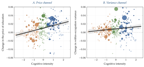
Each point is a three-digit occupation, plotted against the occupation’s Autor and Dorn (2013) measure of cognitive task intensity. Panel A plots the 1980–2010 change in the within-occupation price of education \(\beta_{j}^{\rm edu}\). Panel B plots the change in the within-occupation variance \(V_{j}\). The weighted fits have gradients \(+0.0061\) (standard error \(0.0011\)) and \(+0.0024\) (standard error \(0.0012\)) respectively. Markers are solid where the change in the price of education is statistically significant, \(|z_j|>2\) and hollow otherwise. Marker color indicates terciles of cognitive task intensity (low, orange; middle, green; high, blue) and marker area is proportional to 1980 employment. The shaded regions are pointwise \(95\%\) confidence bands. The observations outside the frame account for \(0.2\%\) of employment in Panel A (5 occupations) and \(0.3\%\) in Panel B (9 occupations). All occupations are retained in the regressions. Census 1980 and ACS 2010, \(J = 286\) three-digit occupations observed in both years.
B.7 Robustness to the Treatment of Self-Employment
Our basic Census and ACS samples retain self-employed workers reporting positive wage and salary income. Table B.5 reports the within/between variance decomposition from Table 1 under two alternative treatments of self-employment: (i) dropping the unincorporated self-employed, whose earnings are largely reported as business rather than wage income, and (ii) dropping all self-employed workers.
| Raw | Residual | |||
|---|---|---|---|---|
| Total | Between | Within | Within | controls | |
| Basic sample | ||||
| 1980 | 0.351 | 0.082 | 0.268 | 0.240 |
| 2010 | 0.407 | 0.121 | 0.286 | 0.270 |
| Change | 0.056 | 0.038 | 0.017 | 0.031 |
| Excluding unincorporated self-employed | ||||
| 1980 | 0.344 | 0.082 | 0.261 | 0.232 |
| 2010 | 0.402 | 0.120 | 0.282 | 0.266 |
| Change | 0.058 | 0.038 | 0.021 | 0.034 |
| Excluding all self-employed | ||||
| 1980 | 0.332 | 0.080 | 0.253 | 0.225 |
| 2010 | 0.390 | 0.119 | 0.271 | 0.255 |
| Change | 0.057 | 0.039 | 0.018 | 0.030 |
Within- and between-occupation decomposition of the variance of log
wages under alternative treatments of self-employment. The basic sample,
used throughout the paper, retains self-employed workers reporting
positive wage and salary income. The second panel additionally excludes
the unincorporated self-employed, whose earnings are largely reported as
business rather than wage income. The third panel excludes all
self-employed workers. The basic sample covers \(J=290\) three-digit occupations. In each
restricted sample the exclusion is applied before the
hundred-observation threshold, and both restrictions remove the same
single occupation, leaving \(J=289\).
Residual wages control for gender, race and hours with
occupation-specific coefficients. Census 1980 and ACS 2010,
occ1990dd occupations with at least 100 observations in
both years, weighted by 1980 employment shares.
The change in residual within-occupation inequality is \(+0.031\) in the basic sample, \(+0.034\) under treatment (i) dropping the unincorporated, and \(+0.030\) under treatment (ii) dropping all self-employed. We find that the levels of inequality are more sensitive than the changes are to how we treat self-employment. Excluding all self-employed workers lowers within-occupation inequality by roughly six percent in both years.
The incorporated self-employed draw wage income from their own businesses and are concentrated in occupations like physicians, dentists and lawyers, where they reach over half of employment in 2010. Excluding them would estimate within-occupation dispersion in those occupations from an unrepresentative minority of professionals who are employees. The unincorporated self-employed, by contrast, are almost entirely one occupation: in 1980 they are 99.8% of employment among farmers, whose measured hourly wage is a secondary wage income divided by total hours worked, giving a within-occupation variance of log wages of 1.26 against 0.27 for the sample as a whole. Either restriction removes the farmer cell entirely and no other, since it falls below the hundred-observation threshold once the unincorporated are dropped.
C Theoretical Results
We first show in Appendix C.1 the equivalence of the direct planning problem, stated in terms of the individual-level bundling constraints, and the indirect planning problem, stated in terms of the aggregate bundling constraint, for the case of \(J=2\) occupations. We then show in Appendix C.2 how our characterization of the aggregate bundling constraint can be extended to \(J\geq2\) occupations. We provide the proofs of our main results in Appendix C.3 and collect miscellaneous additional derivations in Appendix C.4.
Maintained assumptions. Without loss of generality we can name workers \(i\in[0,1]\) so that they are ordered in terms of comparative advantage. We choose this ordering so that \(x(i)/y(i)\) is decreasing, as in the main text. We further assume that the joint distribution of worker types \(H(x,y)\) is smooth in the sense that it has a continuous density that is strictly positive on \(\mathbb{R}^2_{++}\). This ensures that the distribution of comparative advantage \(r=x/y\) has no atoms and no gaps in its support and that the function \(r(i)=x(i)/y(i)\) is continuous and strictly decreasing. Finally, we assume that it is never optimal to shut down an occupation entirely, so that every occupation employs some workers.
C.1 Equivalence of Direct and Indirect Planning Problems
The main text characterizes the efficient allocation using the indirect planning problem, stated in terms of aggregate skills and the aggregate bundling constraint \[ \mathcal{B}:=\bigg\{ \; (X,Y)\in \mathcal{E} \; : \; Y\in[\,\underline{B}(X)\,,\,\overline{B}(X)\,]\; \bigg\}\] In this appendix we show that this problem is equivalent to the direct planning problem, stated in terms of individual-level bundling constraints. We start with the properties of the boundaries \(\underline{B}(X),\overline{B}(X)\) of the aggregate bundling constraint.
Properties of the boundaries. For any \(X\in[0,\overline{X}]\) let \(i^*(X)\) and \(i^{**}(X)\) solve \[\tag{C.1} \int_0^{i^*(X)} x(i)\,di = X= \int_{i^{**}(X)}^1 x(i)\,di\] The former obtains \(X\) from the workers with the highest comparative advantage ratio \(x(i)/y(i)\) moving down, the latter obtains \(X\) from the workers with the lowest comparative advantage ratio \(x(i)/y(i)\) moving up. Then let \[\tag{C.2} \underline{B}(X):=\int_0^{i^*(X)} y(i)\,di,\qquad \overline{B}(X):=\int_{i^{**}(X)}^1 y(i)\,di\] denote the levels of \(Y\) implied by these ways of obtaining \(X\). We then have:
Lemma C.1 (Boundaries). Let \(S\subseteq[0,1]\) be any set of workers such that \[ \int_S x(i)\,di = X\]
The amount of \(Y\) associated with these workers is bounded by \[\tag{C.3} \underline{B}(X)\;\leq\;\int_S y(i)\,di\;\leq\;\overline{B}(X)\] The lower bound holds with equality if and only if \(S\) coincides with \([0,i^*(X)]\). The upper bound holds with equality if and only if \(S\) coincides with \([i^{**}(X),1]\).
The boundaries \(\underline{B}\) and \(\overline{B}\) are continuous and increasing, with \(\underline{B}(0)=\overline{B}(0)=0\) and \(\underline{B}(\overline{X})=\overline{B}(\overline{X})=\overline{Y}\). Moreover \(\underline{B}\) is strictly convex, \(\overline{B}\) is strictly concave, and both are continuously differentiable on \((0,\overline{X})\) with derivatives \[\tag{C.4} \underline{B}'(X)=\frac{y(i^*(X))}{x(i^*(X))},\qquad \overline{B}'(X)=\frac{y(i^{**}(X))}{x(i^{**}(X))}\] Hence \(\mathcal{B}\) is a convex, compact subset of \(\mathcal{E}\).
Proof. Recall that \(r(i):=x(i)/y(i)\) is strictly decreasing in \(i\). To simplify notation let \(i^*=i^*(X)\), \(S^*=[0,i^*]\) and \(r^*=r(i^*)\). For part (i), by construction \(S\) and \(S^*\) deliver the same \(X\), so removing their common part leaves \[ \int_{S\setminus S^*} x(i)\,di - \int_{S^*\setminus S} x(i)\,di = 0\] For workers \(i\in S\setminus S^*\) we have \(i>i^*\), hence \(r(i)<r^*\), hence \(x(i)<r^*y(i)\). For workers \(i\in S^*\setminus S\) we have \(i\leq i^*\), hence \(r(i)\geq r^*\), hence \(x(i)\geq r^*y(i)\). Therefore \[ r^*\Big(\int_{S\setminus S^*}y(i)\,di-\int_{S^*\setminus S}y(i)\,di\Big) \;\geq\;\int_{S\setminus S^*}x(i)\,di-\int_{S^*\setminus S}x(i)\,di=0\] Dividing by \(r^*>0\) and adding \(\int_{S\cap S^*}y(i)\,di\) to both sides gives \(\int_S y(i)\,di\geq\int_{S^*}y(i)\,di=\underline{B}(X)\), the lower bound in (C.3). Since \(r(i)\) is strictly decreasing, the inequalities \(x(i)<r^*y(i)\) for \(i>i^*\) and \(x(i)>r^*y(i)\) for \(i<i^*\) are strict, so equality holds only if \(S\setminus S^*\) and \(S^*\setminus S\) are both null, i.e., only if \(S\) coincides with \(S^*\). The upper bound is the mirror image with \(i^{**}\), \(S^{**}=[i^{**},1]\) and \(r^{**}=r(i^{**})\), and the inequalities reversed.
For part (ii), we have from (C.1) that \(i^*(X)\) is increasing in \(X\) with \(i^*(0)=0\) and \(i^*(\overline{X})=1\), so \(\underline{B}\) is increasing with \(\underline{B}(0)=0\) and \(\underline{B}(\overline{X})=\overline{Y}\). For \(X<X'\) the increment \(\underline{B}(X')-\underline{B}(X)=\int_{i^*(X)}^{i^*(X')}y(i)\,di\) involves workers with \(r(i)\) between \(r(i^*(X'))\) and \(r(i^*(X))\), and \(\int_{i^*(X)}^{i^*(X')}x(i)\,di=X'-X\), so the difference quotients are bounded by \[\tag{C.5} \frac{1}{r(i^*(X))}\;\leq\;\frac{\underline{B}(X')-\underline{B}(X)}{X'-X}\;\leq\;\frac{1}{r(i^*(X'))}\] Since \(r(i^*(X))\) is continuous in \(X\), taking \(X'\rightarrow X\) from either side establishes that \(\underline{B}\) is differentiable, and hence continuous, with \[ \underline{B}'(X)=\frac{1}{r(i^*(X))}=\frac{y(i^*(X))}{x(i^*(X))}\] which is the first part of (C.4). Since \(r(i^*(X))\) is continuous and strictly decreasing, \(\underline{B}(X)\) is continuously differentiable, strictly increasing, and strictly convex. The properties of \(\overline{B}(X)\) follow from the mirror-image arguments with \(i^{**}\) in place of \(i^*\) and the ordering reversed. Finally, \(\mathcal{B}\) is the intersection of the epigraph of \(\underline{B}(X)\), the subgraph (hypograph) of \(\overline{B}(X)\), and the Edgeworth box \(\mathcal{E}\). The first is convex because \(\underline{B}(X)\) is convex, the second because \(\overline{B}(X)\) is concave, and the intersection of convex sets is convex. It is closed because \(\underline{B}(X)\) and \(\overline{B}(X)\) are continuous and bounded because it lies in \(\mathcal{E}:=[0,\overline{X}]\times[0,\overline{Y}]\), hence compact, and it is non-empty because \(\underline{B}(X)\leq\overline{B}(X)\) by part (i). ◻
Let \(\phi(i)\in[0,1]\) denote the probability that worker \(i\) is assigned to occupation 1. The direct problem can then be written:
Direct Planning Problem. Choose assignment \(\phi(i)\in[0,1]\) for each \(i\) to maximize \[\tag{C.6} U\big(\, F_1(X_1,Y_1)\, , \,F_2(X_2,Y_2)\, \big)\] subject to \[\tag{C.7} X_1 + X_2\leq \overline{X},\qquad \qquad Y_1+Y_2\leq \overline{Y}\] and \[\tag{C.8} X_{1} = \int_0^1 x(i) \phi(i) \, di,\qquad \qquad Y_{1} = \int_0^1 y(i) \phi(i) \, di\]
Since the objective (C.6) and the aggregate constraints (C.7) are the same as in the indirect planning problem, the key step is to show that the set of feasible aggregates \((X_1,Y_1)\) delivered by some assignment \(\phi:[0,1]\rightarrow[0,1]\) coincides with the aggregate bundling constraint \(\mathcal{B}\). This step is given by:
Lemma C.2 (Feasible aggregates). Let \(\mathcal{F}\subseteq \mathcal{E}\) be the set of pairs \((X_1,Y_1)\) that can be delivered by some assignment \(\phi:[0,1]\rightarrow[0,1]\) with \[ X_{1} = \int_0^1 x(i) \phi(i) \, di,\qquad \qquad Y_{1} = \int_0^1 y(i) \phi(i) \, di\]
The set \(\mathcal{F}=\mathcal{B}\).
Points on the lower boundary \(Y_1=\underline{B}(X_1)\) are delivered by, and only by, the pure assignment \[ \phi(i) = \mathbf{1}\{i\leq i^*(X_1) \}\] Points on the upper boundary \(Y_1=\overline{B}(X_1)\) are delivered by, and only by, the pure assignment \[ \phi(i) = \mathbf{1}\{i\geq i^{**}(X_1) \}\]
Proof. For part (i), we first show \(\mathcal{F}\subseteq \mathcal{B}\) and then \(\mathcal{B}\subseteq \mathcal{F}\). For \(\mathcal{F}\subseteq \mathcal{B}\), fix any assignment \(\phi\) and let \((X_1,Y_1)\) be the aggregates delivered by this assignment. If \(\phi\) is a pure assignment, \(\phi(i)=\mathbf{1}\{i\in S\}\) for some set of workers \(S\), then Lemma C.1 applied to \(S\) gives \(\underline{B}(X_1)\leq Y_1\leq\overline{B}(X_1)\). If \(\phi\) is a mixed assignment, let \(i^*=i^*(X_1)\) and \(r^*=r(i^*)\) as in the proof of Lemma C.1. Then for every \(i\) \[\tag{C.9} \big(\phi(i)-\mathbf{1}\{i\leq i^*\}\big)\big(y(i)-x(i)/r^*\big) \geq0\] since if \(i\leq i^*\) both factors are non-positive and if \(i>i^*\) both factors are non-negative. Integrating over \(i\) then gives \[ Y_1-\underline{B}(X_1)=\int_0^1\big(\phi(i)-\mathbf{1}\{i\leq i^*\}\big)\,y(i)\,di \;\geq\;\frac{1}{r^*}\int_0^1\big(\phi(i)-\mathbf{1}\{i\leq i^*\}\big)\,x(i)\,di=0\] A symmetric argument establishes \(Y_1\leq \overline{B}(X_1)\). Hence \(\mathcal{F}\subseteq\mathcal{B}\).
For \(\mathcal{B}\subseteq \mathcal{F}\), take any \((X_1,Y_1)\in\mathcal{B}\) and consider the two pure assignments \[ \phi^*(i)=\mathbf{1}\{i\leq i^*(X_1)\},\qquad \phi^{**}(i)=\mathbf{1}\{i\geq i^{**}(X_1)\}\] By (C.1)–(C.2) both deliver \(X_1\) units of skill \(X\), and they deliver \(\underline{B}(X_1)\) and \(\overline{B}(X_1)\) units of skill \(Y\) respectively. For probability \(p\in[0,1]\) the mixed assignment \(\phi(i)=p\phi^{*}(i)+(1-p)\phi^{**}(i)\) delivers \(X_1\) units of skill \(X\) and \(p \underline{B}(X_1)+(1-p)\overline{B}(X_1)\) units of skill \(Y\), which ranges over \([\underline{B}(X_1),\overline{B}(X_1)]\) as \(p\) ranges over \([0,1]\). So every point of \(\mathcal{B}\) is delivered by some assignment, \(\mathcal{B}\subseteq\mathcal{F}\). Hence \(\mathcal{F}=\mathcal{B}\).
For part (ii), we have just seen that the assignments \(\phi^{*}(i)\) and \(\phi^{**}(i)\) can deliver the lower and upper boundary points. That they are the only assignments that can do so follows from (C.9). Since \(r(i)\) is strictly decreasing, the integrand is strictly positive wherever \(i\neq i^*\) and \(\phi(i)\neq\mathbf{1}\{i\leq i^*\}\), so \(Y_1=\underline{B}(X_1)\) requires \(\phi(i)\) to coincide with \(\phi^*(i)\). A symmetric argument applies for the upper boundary. ◻
Equivalence. With this result in hand, equivalence between the indirect planning problem and the direct planning problem follows almost immediately. By Lemma C.2 the two problems are the same maximization problem written in terms of different choice variables. The indirect problem maximizes the same objective over the set of aggregate skills that some assignment can deliver and the objective is independent of which assignment is used to deliver a given set of aggregate skills. Hence the two problems have the same value, the aggregates \((X_1,Y_1)\) of any solution to the direct problem solve the indirect problem, and any solution to the indirect problem is delivered by an assignment from Lemma C.2.
With this equivalence result in hand, we conclude this appendix by reviewing some key features of the solution that were passed over lightly in the main text.
Which boundary binds? Let \(\underline{\mu}\geq0\) and \(\overline{\mu}\geq0\) denote respectively the multipliers on the lower boundary constraint \(Y_1\geq\underline{B}(X_1)\) and the upper boundary constraint \(Y_1\leq\overline{B}(X_1)\) in the indirect problem. The only way for both constraints to hold with equality is for \(X_1=0\) or \(X_1=\overline{X}\), meaning one or other of the occupations is completely shut down, which is not optimal. Hence at most one multiplier \(\underline{\mu}\) or \(\overline{\mu}\) is positive. Suppose that \(\overline{\mu}>0\). Then the first order conditions can be written \[ U_1F_{1X}-U_2F_{2X}=-\overline{\mu}\,\overline{B}'(X_1)<0, \qquad U_2F_{2Y}-U_1F_{1Y}=-\overline{\mu}<0\] If so, \(\lambda_{1X}<\lambda_{2X}\) and \(\lambda_{1Y}>\lambda_{2Y}\), meaning that occupation 2 pays more for skill \(X\) and occupation 1 pays more for skill \(Y\). This is ruled out by our labeling convention in the main text: occupation 1 is the occupation that values skill \(X\) more highly, \(\lambda_{1X}\geq\lambda_{2X}\). Intuitively, if occupations are labeled such that occupation 1 is the more skill \(X\) intensive occupation, the potentially binding boundary constraint is the lower boundary, the one that is activated by attempting to assign ‘too much’ \(X\) relative to \(Y\) to occupation 1. Accordingly, we write \(\mu=\underline{\mu}\), giving (12)–(13) in the main text.
Assignment and the marginal worker. The Lagrangian of the direct problem, with \(\lambda_{jX}:=U_jF_{jX}\) and \(\lambda_{jY}:=U_jF_{jY}\), is linear in \(\phi(i)\). The planner sets \(\phi(i)=1\) if and only if \[\tag{C.10} \lambda_{1X}x(i)+\lambda_{1Y}y(i)\;\geq\;\lambda_{2X}x(i)+\lambda_{2Y}y(i) \qquad\Longleftrightarrow\qquad r(i)\;\geq\;r^*:=\frac{\lambda_{2Y}-\lambda_{1Y}}{\lambda_{1X}-\lambda_{2X}}\] whenever \(\lambda_{1X}>\lambda_{2X}\) and \(\lambda_{2Y}>\lambda_{1Y}\), and is indifferent about every worker when the two occupations have the same skill prices. In the bundled case, \(\mu>0\), the first-order conditions of the indirect problem give \[\tag{C.11} \underline{B}'(X_1)=\frac{U_1F_{1X}-U_2F_{2X}}{U_2F_{2Y}-U_1F_{1Y}}=\frac{\lambda_{1X}-\lambda_{2X}}{\lambda_{2Y}-\lambda_{1Y}}=\frac{1}{r^*}\] From (C.4) we then have \(\underline{B}'(X_1)=1/r(i^*(X_1))\), so \(r^*=r(i^*(X_1))\). The cutoff in the direct problem’s assignment rule is the comparative advantage of the marginal worker \(i^*(X_1)\) on the boundary of \(\mathcal{B}\) at the solution of the indirect problem. The two problems select the same marginal worker, and the workers with \(r(i)\geq r^*\) deliver \((X_1,\underline{B}(X_1))\). This is the same marginal worker \(i^*\) from Section 3.1 in the main text. In the unbundled case, \(\mu=0\), the planner is indifferent as to the assignment of individual workers and the aggregates are delivered by any of the assignments in Lemma C.2. In either case, the shadow prices \(\lambda_{jX},\lambda_{jY}\), and hence the marginal values \(\Lambda_j(x,y)\), coincide across the two formulations.
Indeterminacy of assignment in an unbundled allocation. If \(\mu=0\) every worker has the same value in both occupations. From Lemma C.2, any interior point of \(\mathcal{B}\) is obtained by many assignments. In such an unbundled allocation, the aggregate amounts of each skill, the output of each occupation — and each worker’s equilibrium wage — are fully determined, but the assignment of individual workers between occupations is not. Any statement about within-occupation inequality in an unbundled equilibrium therefore requires some auxiliary selection rule that specifies the assignment. For example, in the symmetric economy of Section 5.1.2 for any unbundled equilibrium we use sorting on comparative advantage with cutoff \(r^*=1\), i.e., the unique assignment that is selected in every bundled equilibrium of that economy.
C.2 Extension to General \(J\) Occupations
To simplify the exposition, the main text presents results for \(J=2\) occupations and characterizes outcomes using a single aggregate bundling constraint of the form \(\underline{B}(X_1)\leq Y_1\leq \overline{B}(X_1)\). With \(J\geq2\) occupations there is a sequence of \(J-1\) constraints of the same form, one for each boundary between adjacent occupations, once occupations are ordered by the comparative advantage of the workers they employ. Importantly, this sequence of constraints can be built using the same functions \(\underline{B}(X), \overline{B}(X)\) from the two-occupation economy, as characterized in Lemma C.1.
Cumulative bundling constraints. Let there be \(J\geq2\) occupations. Let \(S_j\) denote the set of workers assigned to occupation \(j\) by any pure assignment and let \(X_j,Y_j\) denote the aggregate amounts of each skill delivered by that assignment \[ X_j=\int_{S_j}x(i)\,di,\qquad Y_j=\int_{S_j}y(i)\,di\] Then let \(X^{(k)}\) and \(Y^{(k)}\) denote the cumulative aggregate amounts of each skill given by \[\tag{C.12} X^{(k)}:=\sum_{j=1}^k X_j,\qquad Y^{(k)}:=\sum_{j=1}^k Y_j,\qquad k=1,\dots,J\] These are the total amounts of skill \(X\) and skill \(Y\) delivered by the workers in occupations \(j=1,\dots,k\) taken together, that is, by the set of workers \(S^{(k)}:=S_1\cup \cdots \cup S_k\). Applying Lemma C.1 to the set \(S^{(k)}\) then gives \[\tag{C.13} \underline{B}\big(X^{(k)}\big)\;\leq\;Y^{(k)}\;\leq\;\overline{B}\big(X^{(k)}\big),\qquad k=1,\dots,J-1\] with the constraint for \(k=J\) holding automatically since \((X^{(J)},Y^{(J)})=(\overline{X},\overline{Y})\). The allocation of aggregate skills across occupations induced by any assignment must satisfy these \(J-1\) constraints. Note that the functions \(\underline{B}(X)\) and \(\overline{B}(X)\) are the same boundary functions as in the \(J=2\) occupation case, just evaluated at the boundaries between adjacent occupations. By Lemma C.1, the lower constraint in (C.13) holds with equality if and only if \(S^{(k)}=[0,i^*(X^{(k)})]\), that is, if and only if the workers in occupations \(\{1,\dots,k\}\) are precisely those with the highest comparative advantage in \(X\). The same applies symmetrically for the upper constraint.
Importantly, these properties of the cumulative bundling constraints hold for any labeling of occupations.
Planning problem with \(J\) occupations. Given a labeling of occupations, the planner chooses \(\{X_j,Y_j\}_{j=1}^J\) to maximize \[\tag{C.14} U\big(F_1(X_1,Y_1),\dots,F_J(X_J,Y_J)\big)\] subject to the resource constraints \(\sum_j X_j \leq \overline{X}\) and \(\sum_j Y_j \leq \overline{Y}\) and the \(J-1\) lower cumulative constraints \[\tag{C.15} Y^{(k)}\geq\underline{B}\big(X^{(k)}\big),\qquad k=1,\dots,J-1\] This is the \(J\)-occupation counterpart of the indirect planning problem characterized in the main text. The upper constraints in (C.13) are omitted for the same reason as in the \(J=2\) case, as discussed in Appendix C.1 above. By Lemma C.1 this is a concave program over a convex set, so the Kuhn-Tucker conditions are necessary and sufficient. Let \(\mu_k\geq0\) denote the multipliers on the cumulative constraints and, as in the main text, let \(\lambda_{jX}:=U_jF_{jX}\) and \(\lambda_{jY}:=U_jF_{jY}\) denote the shadow prices of skills in occupation \(j\), evaluated at the solution. Since \(X_j\) and \(Y_j\) enter every cumulative constraint with \(k\geq j\), the first-order conditions for adjacent occupations \(j\) and \(j+1\) differ only in the \(j\)th constraint. Differencing them gives \[\tag{C.16} \lambda_{jX}-\lambda_{j+1,X}=\mu_j\,\underline{B}'\big(X^{(j)}\big),\qquad \lambda_{j+1,Y}-\lambda_{jY}=\mu_j,\qquad j=1,\dots,J-1\] For \(J=2\) these are exactly the first order conditions given in (12)–(13).
We make use of two features of this set of optimality conditions. First, since \(\mu_j\geq0\) and \(\underline{B}'(X)>0\) the solution to the planner’s problem is characterized by a weakly decreasing sequence \(\lambda_{jX}\geq \lambda_{j+1,X}\) and a weakly increasing sequence \(\lambda_{jY}\leq \lambda_{j+1,Y}\). Second, from occupation \(j\) to occupation \(j+1\) the price of skill \(X\) falls and the price of skill \(Y\) rises if and only if the \(j\)th constraint binds, \(\mu_j>0\). If this constraint is slack, occupations \(j\) and \(j+1\) have the same skill prices and workers will be indifferent between those occupations. An unbundled allocation of the \(J\geq2\) economy occurs when every constraint is slack so that skill prices are equalized across all occupations, and a fully bundled allocation occurs when every constraint binds.
Sorting on comparative advantage. Now consider how best to assign workers across occupations so as to deliver the planner’s desired aggregate skills. The marginal value to the planner of assigning worker \(i\) to occupation \(j\) is \(\Lambda_j(x(i),y(i))=\lambda_{jX}x(i)+\lambda_{jY}y(i)\) where \(\lambda_{jX},\lambda_{jY}\) are the shadow prices of the aggregate skills in occupation \(j\). Again using \(r(i)=x(i)/y(i)\) to denote a worker’s comparative advantage in \(X\)-intensive occupations, worker \(i\) is assigned to the occupation \(j\) that maximizes \[ \lambda_{jX}\,r(i) + \lambda_{jY}\] Each occupation is represented by a straight line in \(r\) with positive slope \(\lambda_{jX}\) and positive intercept \(\lambda_{jY}\). Worker \(i\) is represented by a vertical line at \(r=r(i)\), and the planner picks for them the occupation \(j\) whose line is highest there. The upper envelope of these lines is convex, so as \(r(i)\) falls workers are assigned to occupations with lower slopes, i.e., lower \(\lambda_{jX}\), and hence higher \(j\), by equation (C.16).
This means workers with the strongest comparative advantage in \(X\)-intensive occupations are assigned to occupation \(j=1\) and those with the strongest comparative advantage in \(Y\)-intensive occupations are assigned to occupation \(j=J\). Any two occupations \(j\) and \(j+1\) such that \(\mu_j=0\) have the same line and hence workers would be indifferent between those two occupations. In solving the sorting problem, we collapse such occupations so that across every remaining boundary both wedges in (C.16) are strictly positive.
Now for every remaining boundary let \(r_j^*\) denote the comparative advantage of a worker who would be just indifferent between occupations \(j\) and \(j+1\), that is, \[\tag{C.17} r_j^*=\frac{\lambda_{j+1,Y}-\lambda_{jY}}{\lambda_{jX}-\lambda_{j+1,X}}=\frac{1}{\underline{B}'\big(X^{(j)}\big)}>0\] where the second equality follows from (C.16). For completeness also set \(r_0^*=+\infty\) and \(r_J^*=0\). Since \(\underline{B}'(X)\) is strictly increasing and \(X^{(j)}\) is increasing in \(j\), these cutoffs form a strictly decreasing sequence \(r_0^*>r_1^*>\cdots>r_J^*\). Since the upper envelope of lines is convex, each occupation’s line is highest on an interval of \(r\) and these intervals are arranged in order of \(j\). The planner therefore allocates all workers with \(r(i)\in(r^*_j,r^*_{j-1})\) to occupation \(j\). In particular, since \(r(i)\) is strictly decreasing in \(i\), the workers allocated to occupations \(\{1,\dots,k\}\) are precisely the workers with \(r(i)\geq r_k^*\), i.e., the workers with the highest comparative advantage in \(X\).
Equivalence with \(J\) occupations. The direct problem with \(J\) occupations chooses a pure assignment of workers to occupations to maximize (C.14), with \(X_j\) and \(Y_j\) the aggregates the assignment delivers to occupation \(j\). The indirect problem is (C.14)–(C.15). Now consider the fully bundled case, \(\mu_k>0\) for \(k=1,\dots,J-1\), so that the sorting pattern above applies to all \(J\) occupations. From (C.4), the second equality in (C.17) implies that \(r_k^*=r(i^*(X^{(k)}))\), i.e., the worker who would be just indifferent between occupations \(k\) and \(k+1\) is the boundary worker \(i^*(X^{(k)})\) from Lemma C.1, evaluated at the planner’s cumulative allocation. This is the \(J\)-occupation version of our familiar condition (C.11) characterizing the marginal worker, except now there is one such condition for each boundary. Hence the workers allocated to occupations \(\{1,\dots,k\}\) are precisely the set \([0,i^*(X^{(k)})]\), which delivers \(X^{(k)}\) units of skill \(X\) and \(\underline{B}(X^{(k)})\) units of skill \(Y\), and \(\underline{B}(X^{(k)})=Y^{(k)}\) since the \(k\)th constraint binds. Since this holds at every boundary, the sorting pattern delivers the planner’s cumulative aggregates \((X^{(k)},Y^{(k)})\) for every \(k\) and hence the planner’s \((X_j,Y_j)\) for every \(j\). Conversely, the aggregates delivered by any assignment satisfy (C.13), so the value of the indirect problem is an upper bound on the value of the direct problem, and the sorting pattern attains that upper bound. Hence the two problems coincide, exactly as in Appendix C.1. If instead some constraints are slack, the economy is bundled across some boundaries and not others — adjacent occupations with \(\mu_k=0\) share both skill prices, the planner is indifferent about how their workers are divided between them, and the sorting pattern applies to the set of collapsed occupations.
Finally, summing (C.16) gives \[\tag{C.18} \lambda_{jX}=\lambda_{1X}-\sum_{k=1}^{j-1}\mu_k\,\underline{B}'\big(X^{(k)}\big)=\lambda_{1X}-\sum_{k=1}^{j-1}\frac{\mu_k}{r_k^*}\] The price of skill \(X\) in occupation \(j\) is its price in the most \(X\)-intensive occupation less the accumulated bundling wedges at each boundary in between, each divided by the comparative advantage of the marginal worker at that boundary. This is the finite-\(J\) counterpart of the expression for skill prices in the model of one-to-one matching with a continuum of occupations in Section 4.3.
Continuum of occupations. The one-to-one assignment model of Section 4.3 is the limit of the \(J\)-occupation problem as occupations become dense. To obtain this limit we place occupations on a grid \(j=k/J\), \(k=1,\dots,J\), with spacing \(\Delta:=1/J\), and write \(X_k=X(j)\Delta\), \(Y_k=Y(j)\Delta\) and \(\mu_k=\mu(j)\Delta\). The cumulative aggregates (C.12) become \(X^{(j)}=\int_0^j X(j')\,dj'\) and \(Y^{(j)}=\int_0^j Y(j')\,dj'\), and the cumulative constraints (C.15) become \(Y^{(j)}\geq\underline{B}(X^{(j)})\) for all \(j\in[0,1]\), with the same boundary function \(\underline{B}(X)\). Dividing the wedge conditions (C.16) by \(\Delta\) and letting \(\Delta\to0\) gives \[ \frac{d\lambda_X(j)}{dj}=-\mu(j)\,\underline{B}'\big(X^{(j)}\big) =-\mu(j)\,\frac{y(i^*(j))}{x(i^*(j))},\qquad \frac{d\lambda_Y(j)}{dj}=\mu(j)\] where \(i^*(j):=i^*(X^{(j)})\) is the marginal worker at boundary \(j\). When \(\mu(j)>0\) for all \(j\), every constraint binds, \(j\mapsto i^*(j)\) is strictly increasing, and its inverse \(j^*(i)\) is the occupation of worker \(i\), as used in Section 4.3. In this case sorting is one-to-one. On any interval where \(\mu(j)=0\), skill prices are constant, workers are indifferent among those occupations, and the assignment among them is indeterminate, exactly as for the collapsed occupations (if any) in the finite-\(J\) case. Integrating the first equation from \(j=0\) gives the expression for \(\lambda_X(j)\) in equation (32), the continuum counterpart of (C.18) above.
C.3 Proofs of Main Results
Proof of Proposition 1.
We first show that any competitive equilibrium allocation solves the indirect planning problem with wages \(W_j(x,y)=\Lambda_j(x,y)\). We then show that any solution to the planning problem can be decentralized as a competitive equilibrium.
Equilibrium conditions. Let the final good be the numeraire and let \(P_j\) denote the price of output from occupation \(j\) in final good units. The final good is produced by many identical perfectly competitive firms with the technology \(U\). Profit maximization by the final good producers gives the standard condition \(U_j=P_j\). Taking wages \(W_j(x,y)\) and prices \(P_j\) as given, the representative firm in occupation \(j\) hires labor \(L_j(x,y)\) to \[ \min_{L_j}\int W_j(x,y)\,dL_j(x,y)\qquad\text{subject to}\qquad\int x\,dL_j(x,y)=X_j,\qquad\int y\,dL_j(x,y)=Y_j\] Let \(\lambda_{jX},\lambda_{jY}\) denote the multipliers on these two constraints. Both the objective and the constraints are linear in \(L_j(x,y)\), so the firm hires type \((x,y)\) only if \(W_j(x,y)\leq\lambda_{jX}x+\lambda_{jY}y\), demands an unlimited amount of that type if the inequality is strict, and is indifferent if it holds with equality. In equilibrium, therefore, every type the firm hires is paid exactly \[ W_j(x,y)=\lambda_{jX}\,x+\lambda_{jY}\,y=\Lambda_j(x,y)\] and the firm’s total cost is \(\lambda_{jX}X_j+\lambda_{jY}Y_j\). Profit maximization over \((X_j,Y_j)\) then gives \(\lambda_{jX}=P_jF_{jX}\) and \(\lambda_{jY}=P_jF_{jY}\), with zero profits by constant returns to scale. Hence \[\tag{C.19} \lambda_{jX}=U_jF_{jX},\qquad \lambda_{jY}=U_jF_{jY}\] which are the planner’s shadow prices evaluated at the equilibrium aggregates. Finally, each worker chooses the occupation with the highest wage, \(\max_j W_j(x,y)=\max_j\Lambda_j(x,y)\), which gives the same assignment rule as in equation (C.10).
Equilibrium allocation is efficient. Take any competitive equilibrium and label occupations so that \(\lambda_{1X}\geq\lambda_{2X}\). There are two cases to consider. First, if \(\lambda_{1X}=\lambda_{2X}\) then also \(\lambda_{1Y}=\lambda_{2Y}\), since otherwise one occupation would pay more for both skills and the other would employ no workers. Then (C.19) gives (12)–(13) with \(\mu=0\), and the equilibrium aggregates \((X_1,Y_1)\) lie in \(\mathcal{B}\) by Lemma C.2. Second, if instead \(\lambda_{1X}>\lambda_{2X}\) then \(\lambda_{1Y}<\lambda_{2Y}\) by the same argument, and workers sort according to (C.10) with cutoff \(r^*\in(0,\infty)\). Occupation 1 then employs exactly the workers with \(r(i)\geq r^*\), i.e., the set \([0,i^*(X_1)]\), so by Lemma C.1 \(Y_1=\underline{B}(X_1)\) and \(\underline{B}'(X_1)=1/r^*\). Setting \(\mu:=\lambda_{2Y}-\lambda_{1Y}>0\) and using (C.19), the conditions (12)–(13) hold with the bundling constraint binding. In both cases the equilibrium aggregates satisfy the Kuhn-Tucker conditions of the indirect problem. Since this is a concave program over the convex set \(\mathcal{B}\), by Lemma C.1, these conditions are sufficient, so the equilibrium allocation is efficient.
Efficient allocation can be decentralized. Conversely, take a solution \((X_j,Y_j)\) to the indirect planning problem with multiplier \(\mu\geq0\) and construct prices from the planner’s shadow values: let \(P_j:=U_j\), \(\lambda_{jX}:=U_jF_{jX}\) and \(\lambda_{jY}:=U_jF_{jY}\), and set wages \(W_j(x,y):=\Lambda_j(x,y)=\lambda_{jX}x+\lambda_{jY}y\), all evaluated at the planner’s solution. Then from the equilibrium conditions in Section 3.2 we have:
Final good producers. Prices satisfy \(P_j=U_j\) by construction.
Occupations. At wages \(W_j(x,y)=\Lambda_j(x,y)\) a firm is indifferent over which types \((x,y)\) it hires, and any plan delivering \((X_j,Y_j)\) costs \(\lambda_{jX}X_j+\lambda_{jY}Y_j\). Moreover since \(\lambda_{jX}=P_jF_{jX}\) and \(\lambda_{jY}=P_jF_{jY}\), the planner’s \((X_j,Y_j)\) satisfies each firm’s first-order conditions, and, by constant returns, each firm earns zero profits at any scale.
Workers. Each worker chooses occupation \(j\) to maximize \(\Lambda_j(x,y)\). If \(\mu>0\), this is the cutoff rule (C.10) with \(r^*=r(i^*(X_1))\) by (C.11), and, by part (ii) of Lemma C.2, this assignment delivers exactly \((X_1,\underline{B}(X_1))=(X_1,Y_1)\), and hence \((X_2,Y_2)\). If \(\mu=0\), skill prices are equalized across occupations, every worker is indifferent, and, by part (i) of Lemma C.2, some assignment delivers \((X_1,Y_1)\). Any such assignment is consistent with worker optimality.
In either case, \(\mu>0\) or \(\mu=0\), the assignment delivers the aggregates that firms demand, so skill markets clear, and the final good market clears by Walras’ law. Hence the efficient allocation is a competitive equilibrium, with wages \(W_j(x,y)=\Lambda_j(x,y)\). \(\square\)
Proof of Lemma 1.
To simplify notation, write \(\beta:=\beta_{jX}\), so that \(\beta_{jY}=1-\beta\), and drop the \(j\) subscript on the moments of the skill distribution. Then substituting \(\ln x=\ln r+\ln y\) into \(V_j=\text{Var}[\beta\ln x+(1-\beta)\ln y]=\text{Var}[\ln y+\beta\ln r]\) gives \[\tag{C.20} V_j(\beta)=\text{Var}[\ln y]+2\beta\,\text{Cov}[\ln y,\ln r]+\beta^2\,\text{Var}[\ln r]\] which is a convex quadratic in \(\beta\) with \[ \frac{dV_j}{d\beta}=2\big(\beta\,\text{Var}[\ln r]+\text{Cov}[\ln y,\ln r]\big)\] This is positive if and only if \(\beta>-\text{Cov}[\ln y,\ln r]/\text{Var}[\ln r]=\beta^*_{jX}\). Finally, from (19), \(\beta/(1-\beta)=(\lambda_{jX}/\lambda_{jY})(\overline{x}_j/\overline{y}_j)\), so holding the composition of the occupation fixed, \(\beta\) is a strictly increasing function of the skill price gradient \(\lambda_{jX}/\lambda_{jY}\). Hence \(V_j\) is increasing in the skill price gradient if and only if \(\beta_{jX}>\beta^*_{jX}\). \(\square\)
Properties of the symmetric economy. The proofs of Proposition 2 and Proposition 3 below use the following properties of the Symmetric Economy special case of our main specification with Cobb-Douglas technologies and IID Fréchet skills:
Since both skills have the same Fréchet shape \(\theta\) and, given \(\overline{X}=\overline{Y}\), the same scale, the joint distribution of skills \((x,y)\) is unchanged if the skills are exchanged, \((x,y)\mapsto(y,x)\), so that the index of comparative advantage \(r\mapsto 1/r\).
The set \(\mathcal{B}\) is symmetric about the off-diagonal \(Y_1=\overline{X}-X_1\) of the Edgeworth box \(\mathcal{E}\). Exchanging the two skills and exchanging the two occupations maps a set of workers delivering \((X_1,Y_1)\) to a set of workers delivering \((\overline{X}-Y_1,\overline{X}-X_1)\). Hence \((X_1,Y_1) \in \mathcal{B}\) if and only if \((\overline{X}-Y_1,\overline{X}-X_1)\in \mathcal{B}\) and the same exchange map sends the lower boundary of \(\mathcal{B}\) to itself.
With the symmetric Cobb-Douglas technologies, exchanging skills and occupations leaves the planner’s objective unchanged.
The solution to the indirect problem is unique since the objective is strictly concave in \((X_1,Y_1)\) and \(\mathcal{B}\) is convex by Lemma C.1. Since a unique solution to a symmetric problem must be a fixed point of the exchange map, the solution lies on the off-diagonal and to simplify notation we can then write \[ X:= X_1 = Y_2,\qquad \text{and}\qquad X_2 = Y_1 = \overline{X}-X\] for the allocations of the primary skill and the secondary skill, as in Section 5.1.2.
Under symmetry occupation-level output is equalized, \(C_1=C_2\), and we can write \[ U=C_1^{1/2} C_2^{1/2} = F(X):=X^{\alpha} (\overline{X}-X)^{1-\alpha}\] so that \(U_1=U_2=1/2\). Hence the skill prices in this economy are given by \[\tag{C.21} \lambda_{1X}=\lambda_{2Y}=\frac{\alpha}{2}\,\bigg(\frac{F(X)}{X}\bigg),\qquad \lambda_{1Y}=\lambda_{2X}=\frac{1-\alpha}{2}\,\bigg(\frac{F(X)}{\overline{X}-X}\bigg)\] From the planner’s conditions (12)–(13) the multiplier on the bundling constraint is \[\tag{C.22} \mu=\lambda_{2Y}-\lambda_{1Y}=\frac{1}{2}\,F'(X)\] Note that the two first order conditions (12)–(13) reduce to the single condition (C.22) because, from (C.21), the two wedges \(\lambda_{1X}-\lambda_{2X}\) and \(\lambda_{2Y}-\lambda_{1Y}\) are equal. By (C.11) this means \(\underline{B}'(X)=1\): at the symmetric point the marginal worker has \(r^*=1\), i.e., \(x(i^*)=y(i^*)\).
Proof of Proposition 2.
For this symmetric economy the Fréchet lower boundary (8) is \[\tag{C.23} \underline{B}(X)=\bigg(1-\Big(1-\big(X/\overline{X}\big)^{\frac{\theta}{\theta-1}}\Big)^{\frac{\theta-1}{\theta}}\bigg)\,\overline{X}\] This is the expression for \(\underline{B}(X)\) derived in Appendix C.4 below evaluated at \(\overline{X}=\overline{Y}\).
For parts (i) and (ii), the planner maximizes \(F(X)=X^\alpha(\overline{X}-X)^{1-\alpha}\) subject to \((X,\overline{X}-X)\in\mathcal{B}\). The unconstrained maximizer is \(X=\alpha\overline{X}\), which is the unbundled allocation. The unbundled allocation is feasible if and only if \(\overline{X}-\alpha\overline{X}\geq\underline{B}(\alpha\overline{X})\), i.e., if and only if the off-diagonal point with \(X=\alpha\overline{X}\) lies on or above the lower boundary \(\underline{B}(X)\). Now \(X+\underline{B}(X)\) is continuous and strictly increasing in \(X\), from \(0\) at \(X=0\) to \(2\overline{X}\) at \(X=\overline{X}\), so there is a unique \(X^*\) at which \(X^*+\underline{B}(X^*)=\overline{X}\). From (C.23) this requires \((1-(X^*/\overline{X})^{\theta/(\theta-1)})^{(\theta-1)/\theta}=X^*/\overline{X}\), i.e., \(2(X^*/\overline{X})^{\theta/(\theta-1)}=1\), which implies \[ X^*/\overline{X}=\Big(\frac{1}{2}\Big)^{\frac{\theta-1}{\theta}}=:\alpha^*\] Hence the unbundled allocation is feasible if and only if \(\alpha\leq\alpha^*\), giving us part (i). When \(\alpha>\alpha^*\), the off-diagonal meets \(\mathcal{B}\) in the segment \(X\in[(1-\alpha^*)\overline{X},\alpha^*\overline{X}]\), with the lower boundary at the upper end. Since the objective \(F(X)\) is strictly increasing on \([0,\alpha\overline{X}]\) and \(\alpha^*\overline{X}<\alpha\overline{X}\), the constrained maximum is indeed at \(X^*=\alpha^*\overline{X}\), where the lower bundling constraint binds. Writing these two cases out we have (38), which is part (ii).
For part (iii), if \(\alpha\leq \alpha^*\) the constraint is slack and \(\mu=0\). If \(\alpha>\alpha^*\), then from (C.22) we know \(\mu=F'(X)/2\) evaluated at \(X=\alpha^*\overline{X}\). Calculating the marginal product \[ F'(X)=\bigg(\frac{\alpha}{X}-\frac{1-\alpha}{\overline{X}-X}\bigg)\,F(X)\] Evaluating this at \(X=\alpha^*\overline{X}\) and simplifying \[ \mu(\alpha) =\frac{1}{2}\bigg(\frac{\alpha^*}{1-\alpha^*}\bigg)^{\alpha}\bigg(\frac{\alpha-\alpha^*}{\alpha^*}\bigg)\] which is (39). Both factors that depend on \(\alpha\) are positive and strictly increasing on \((\alpha^*,1]\), the first because \(\alpha^*>1/2\), so \(\mu(\alpha)\) is strictly increasing in \(\alpha\), giving us part (iii). \(\square\)
Within-occupation moments. To characterize the distribution of wages when skills \((x,y)\) are IID Fréchet we use some properties of Fréchet and Gumbel random variables that will be familiar from discrete choice models. In what follows we let \(\mathbb{E}_j[X]\), \(\text{Var}_j[X]\), and \(\text{Cov}_j[X,Y]\) denote moments conditional on selection into occupation \(j\). The proof of Proposition 3 uses the following:
Lemma C.3 (Conditional moments). Let \(x,y\) be independent Fréchet with common shape \(\theta>1\) and common scale, and let occupation 1 consist of the workers with \(r=x/y>r^*\). Then:
For any cutoff \(r^*\), \[ \text{Var}_1 [\ln x]=\frac{\pi^2}{6\theta^2}=\text{Var}[\ln x],\qquad \mathbb{E}_1[\ln x]-\mathbb{E}[\ln x]=\frac{\ln(1+r^{*\theta})}{\theta}\]
For the symmetric cutoff \(r^*=1\), \[ \mathbb{E}_1[\ln x-\ln y]=\frac{2\ln2}{\theta},\quad \theta^2\,\text{Var}_1[\ln y]=\frac{\pi^2}{6}-2(\ln2)^2,\quad \theta^2\,\text{Cov}_1[\ln x,\ln y]=(\ln2)^2\] Hence, in terms of comparative advantage \(r\), \[ \theta^2\,\text{Var}_1[\ln r]=\frac{\pi^2}{3}-4(\ln2)^2,\qquad \theta^2\,\text{Cov}_1[\ln y,\ln r]=3(\ln2)^2-\frac{\pi^2}{6}\]
Proof. Without loss of generality set the common scale to one. Then \(G_x:=\theta\ln x\) and \(G_y:=\theta\ln y\) are independent standard Gumbel with mean \(\gamma\) (Euler’s constant) and variance \(\pi^2/6\) and selection into occupation 1 is the event \(\{G_x>G_y+c\}\) with \(c:=\theta\ln r^*\).
For part (i), we use a standard property of independent Gumbel random variables: \(\max\{G_x,G_y+c\}\) is Gumbel with location parameter \(\ln(1+e^{c})\) and is independent of which of the two attains the maximum. Hence, conditional on occupation 1, \(G_x\) is Gumbel with location \(\ln(1+e^c)\) so \(\text{Var}_1[G_x]=\pi^2/6\), the same as unconditionally, and \(\mathbb{E}_1[G_x]=\gamma+\ln(1+e^c)\). Dividing by \(\theta^2\) and \(\theta\) respectively, and using \(e^c=r^{*\theta}\), gives part (i).
For part (ii), \(r^*=1\) implies \(c=0\) so that selection into occupation 1 occurs with probability \(1/2\) and so from part (i) \(\mathbb{E}_1[G_x]=\gamma+\ln2\). Since \(\mathbb{E}[G_y]=\gamma\) is the equally-weighted average of \(\mathbb{E}_1[G_y]\) and \(\mathbb{E}_2[G_y]\), and by symmetry \(\mathbb{E}_2[G_y]=\mathbb{E}_1[G_x]\), we have \(\mathbb{E}_1[G_y]=\gamma-\ln2\), which gives the first claim. For the second moments, the same averaging and symmetry give \[ \mathbb{E}_1[G_y^2]=2\,\mathbb{E}[G_y^2]-\mathbb{E}_1[G_x^2] =2\Big(\frac{\pi^2}{6}+\gamma^2\Big)-\Big(\frac{\pi^2}{6}+(\gamma+\ln2)^2\Big)\] so that \(\text{Var}_1[G_y]=\mathbb{E}_1[G_y^2]-(\gamma-\ln2)^2=\pi^2/6-2(\ln2)^2\). For the covariance, \(\mathbb{E}[G_xG_y]=\gamma^2\) unconditionally and by symmetry \(\mathbb{E}_1[G_xG_y]=\mathbb{E}_2[G_xG_y]\), so both equal \(\gamma^2\) and \(\text{Cov}_1[G_x,G_y]=\gamma^2-(\gamma+\ln2)(\gamma-\ln2)=(\ln2)^2\). The moments in terms of comparative advantage \(r=x/y\) follow from \(\text{Var}_1[\ln r]=\text{Var}_1[\ln x]+\text{Var}_1[\ln y]-2\,\text{Cov}_1[\ln x,\ln y]\) and \(\text{Cov}_1[\ln y,\ln r]=\text{Cov}_1[\ln x,\ln y]-\text{Var}_1[\ln y]\). ◻
Proof of Proposition 3.
Composition. We first pin down the composition of each occupation. From (C.21), in a bundled equilibrium \(\lambda_{1X}=\lambda_{2Y}>\lambda_{1Y}=\lambda_{2X}\) and the cutoff in (C.10) is \[ r^*=\frac{\lambda_{2Y}-\lambda_{1Y}}{\lambda_{1X}-\lambda_{2X}}=1\] So for every \(\alpha>\alpha^*\) occupation 1 consists of the workers with \(r>1\) and occupation 2 of the workers with \(r<1\), each with probability one half. The within-occupation distribution of skills is therefore independent of \(\alpha\) in a bundled equilibrium — in a bundled equilibrium, only the skill prices respond to \(\alpha\). As discussed in Appendix C.1 above, in an unbundled equilibrium the assignment is indeterminate and we fix composition using the same selection rule, sorting on comparative advantage with cutoff \(r^*=1\).
Skill price elasticity. Next we obtain the skill price elasticity. From (C.21) evaluated at \(X=X(\alpha)\), the skill price gradient in occupation 1 is \[ g(\alpha):=\frac{\lambda_{1X}}{\lambda_{1Y}}=\frac{\alpha}{1-\alpha}\, \bigg/ \, \frac{X(\alpha)}{\overline{X}-X(\alpha)}\] which equals \(1\) when \(X(\alpha)=\alpha\overline{X}\) and equals \(\frac{\alpha}{1-\alpha}\big/\frac{\alpha^*}{1-\alpha^*}\) when \(X(\alpha)=\alpha^*\overline{X}\), as in (40). By part (ii) of Lemma C.3, the geometric means of skills within occupation 1 satisfy \[ \ln\overline{x}_1-\ln\overline{y}_1=\mathbb{E}_1[\ln x-\ln y]=2\ln2/\theta\] Hence \(\overline{x}_1/\overline{y}_1=4^{1/\theta}\). Substituting this expression for the ratio of geometric means into (19), the primary skill elasticity is the same in both occupations and equals \[ \beta(\alpha)=\frac{g(\alpha)\,4^{1/\theta}}{g(\alpha)\,4^{1/\theta}+1}\] as in (42) above. Since \(g(\alpha)\geq1\) and \(4^{1/\theta}>1\), we have \(\beta(\alpha)>1/2\) for every \(\alpha\).
Variance of log wages. For any distribution of skills \((x,y)\) the variance of log wages is \[ V_j(\beta_j)=\text{Var}_j[\ln y]+2\beta_j \,\text{Cov}_j[\ln y,\ln r]+\beta_j^2\,\text{Var}_j[\ln r]\] From part (ii) of Lemma C.3 the conditional moments for occupation 1 are \[ \theta^2\,\text{Var}_1[\ln y]=\kappa_0,\qquad 2\theta^2\,\text{Cov}_1[\ln y,\ln r]=\kappa_1,\qquad \theta^2\,\text{Var}_1[\ln r]=\kappa_2\] which are the constants \(\kappa_0,\kappa_1,\kappa_2\) defined in the footnote to (43) in the main text. The same moments hold in occupation 2 with the roles of \(x\) and \(y\) exchanged.
Substituting these constants into our expression for the variance of log wages gives equation (43), common to both occupations, and the threshold from Lemma 1 evaluates to \[ \beta^*=-\frac{\kappa_1}{2\kappa_2}=\frac{\pi^2/6-3(\ln2)^2}{\pi^2/3-4(\ln2)^2}\approx0.149\]
For part (i), if \(\alpha\leq\alpha^*\) then the skill price gradient is \(g(\alpha)=1\), so \(\beta(\alpha)=4^{1/\theta}/(4^{1/\theta}+1)\) depends on \(\theta\) only. With composition fixed at \(r^*=1\), the variance of log wages simplifies to \(V(\alpha)=\overline{V}\) independent of \(\alpha\), where the constant \(\overline{V}\) is (43) evaluated at \(\beta=4^{1/\theta}/(4^{1/\theta}+1)\).
For part (ii), if \(\alpha>\alpha^*\) then the skill price gradient \(g(\alpha)\) is strictly increasing in \(\alpha\) with \(g(\alpha^*)=1\), so \(\beta(\alpha)\) is strictly increasing with \(\beta(\alpha^*)=4^{1/\theta}/(4^{1/\theta}+1)\) and hence \(V(\alpha^*)=\overline{V}\). Since \(\beta(\alpha)>1/2>\beta^*\), Lemma 1 puts the economy on the increasing arm of the quadratic (C.20), so the variance of log wages \(V(\alpha)\) is strictly increasing in \(\alpha\) on \((\alpha^*,1]\). \(\square\)
C.4 Additional Derivations
Fréchet lens boundaries. Suppose skills are independent Fréchet with common shape \(\theta>1\) and scale parameters \(T_X,T_Y>0\), so that \(H(x,y)=H_X(x)H_Y(y)\) with \(H_X(x)=\exp(-T_Xx^{-\theta})\) and \(H_Y(y)=\exp(-T_Yy^{-\theta})\). Writing \(\gamma_{\theta}:=\Gamma(1-1/\theta)\), the aggregate endowments are \(\overline{X}=\gamma_{\theta} T_X^{1/\theta}\) and \(\overline{Y}=\gamma_{\theta} T_Y^{1/\theta}\). In the main text we implicitly choose \(T_X,T_Y\) to set the aggregate endowments \(\overline{X},\overline{Y}\) but for the moment it is more convenient to keep things in the scale parameter form.
A worker is assigned to occupation 1 if their skills \((x,y)\) satisfy \(r=x/y>r^*\) for some cutoff comparative advantage \(r^*\). Integrating over all workers, the total supply of skill \(X\) delivered to occupation 1 is \[ X_1(r^*)=\int_0^\infty x\,H_Y(x/r^*)\,dH_X(x) =\int_0^\infty x\,\theta T_Xx^{-\theta-1}\exp\big(-(T_X+T_Yr^{*\theta})\,x^{-\theta}\big)\,dx\] The integrand is \(T_X/(T_X+T_Yr^{*\theta})\) times \(x\) times the density of a Fréchet distribution with shape \(\theta\) and scale \(T_X+T_Yr^{*\theta}\), so this evaluates to \[ X_1(r^*)=\frac{T_X}{T_X+T_Yr^{*\theta}}\cdot\gamma_{\theta}\,(T_X+T_Yr^{*\theta})^{1/\theta} =\frac{\gamma_{\theta}\,T_X}{(T_X+T_Yr^{*\theta})^{\frac{\theta-1}{\theta}}}\] Likewise the total supply of skill \(Y\) delivered to occupation 1 is \[ Y_1(r^*)=\int_0^\infty y\,\big[1-H_X(yr^*)\big]\,dH_Y(y) =\overline{Y}-\frac{\gamma_{\theta}\,T_Y}{(T_Y+T_Xr^{*-\theta})^{\frac{\theta-1}{\theta}}}\] Using \(\overline{X}=\gamma_{\theta} T_X^{1/\theta}\) and \(\overline{Y}=\gamma_{\theta} T_Y^{1/\theta}\) to write these in terms of the aggregate skill endowments \[\tag{C.24} X_1 \big/ \overline{X}=\bigg(\frac{1}{1+Kr^{*\theta}}\bigg)^{\frac{\theta-1}{\theta}},\qquad Y_1 \big/ \overline{Y} =1-\bigg(\frac{Kr^{*\theta}}{1+Kr^{*\theta}}\bigg)^{\frac{\theta-1}{\theta}}\] where \(K:=(\overline{Y}/\overline{X})^\theta=T_Y/T_X\) denotes the relative scale of the two Fréchet marginals.
To obtain the expression for the lower boundary \(\underline{B}(X)\) we eliminate the cutoff \(r^*\) between the expressions for the aggregate skill endowments in (C.24) using \(Kr^{*\theta}/(1+Kr^{*\theta})=1-(X_1/\overline{X})^{\theta/(\theta-1)}\) which leaves us with \[ Y_1 = \bigg(1-\Big(1-\Big(X_1\big/\overline{X}\Big)^{\frac{\theta}{\theta-1}}\Big)^{\frac{\theta-1}{\theta}}\bigg)\cdot \overline{Y}\] as in equation (8) in the main text. A symmetric argument that starts by assigning the workers with \(r<r^*\) to occupation 1 gives the counterpart upper boundary \(\overline{B}(X)\). Both boundaries are strictly increasing from \(\underline{B}(0)=\overline{B}(0)=0\) to \(\underline{B}(\overline{X})=\overline{B}(\overline{X})=\overline{Y}\) and, since \(\theta>1\), \(\underline{B}(X)\) is strictly convex while \(\overline{B}(X)\) is strictly concave.
Two other properties of this distribution are useful. First, the share of workers in occupation 1 is \[ \text{Prob}[r>r^*] = \frac{1}{1+K r^{* \theta}}\] since \(r\) is log-logistic with shape \(\theta\) and scale \(K^{-1/\theta}\). In the symmetric case with \(\overline{X}=\overline{Y}\) we have \(K=1\) and \(r^*=1\) so this simplifies to a probability of 1/2, as used in the proof of Proposition 3. Second, differentiating the lower boundary, again in the symmetric case with \(\overline{X}=\overline{Y}\), gives \[ \underline{B}'(X)=\bigg(\frac{(X/\overline{X})^{\theta/(\theta-1)}}{1-(X/\overline{X})^{\theta/(\theta-1)}}\bigg)^{1/\theta}=\frac{1}{r^*}\] which recovers the result that the slope of the boundary is given by the comparative advantage \(r^*=r(i^*)\) of the marginal worker, as in (C.4), and in particular equals \(1\) in a bundled equilibrium where \(X=\alpha^*\overline{X}\) and \(r^*=1\), consistent with the proof of Proposition 2.
Cobb-Douglas-Fréchet details. Recall the model of Section 5.1 with asymmetric Cobb-Douglas technologies and independent Fréchet skills with common shape parameter \(\theta\) and aggregate skill endowments \(\overline{X},\overline{Y}\). Let \(s_1:=X_1/\overline{X}\) and \(s_2:=Y_2/\overline{Y}\) denote the shares of each occupation’s primary skill in the unbundled allocation, which work out to be \[ s_1=\frac{\eta_1\alpha_1}{\eta_1\alpha_1+\eta_2\alpha_2},\qquad s_2=\frac{\eta_2(1-\alpha_2)}{\eta_1(1-\alpha_1)+\eta_2(1-\alpha_2)}\] as in (35). Substituting these shares into the Fréchet lower boundary (8) and simplifying we find that \(Y_1\geq \underline{B}(X_1)\) if and only if \[\tag{C.25} \mathcal{T}(s_1,s_2):=\Big(s_1^{\frac{\theta}{\theta-1}}+s_2^{\frac{\theta}{\theta-1}}\Big)^{\frac{\theta-1}{\theta}}\;\leq\;1\] This is a CES aggregator and, since \(\theta>1\), is convex in the primary shares. It has the familiar CES limits \(\mathcal{T}(s_1,s_2)\rightarrow s_1+s_2\) as \(\theta\rightarrow\infty\) (when there is no dispersion in Fréchet draws) and at the other extreme \(\mathcal{T}(s_1,s_2)\rightarrow\max\{s_1,s_2\}<1\) as \(\theta\rightarrow1\) (when there is maximal dispersion in Fréchet draws). More precisely \(\mathcal{T}\) is the \(\ell^p\) norm of \((s_1,s_2)\) with \(p=\theta/(\theta-1)>1\). Three properties follow from this. First, \(\mathcal{T}\) is strictly increasing in each primary share and both \(s_1\) and \(s_2\) are strictly increasing in \(\alpha_1\). At \(\alpha_1=\alpha_2\) we have \(s_1=\eta_1\) and \(s_2=\eta_2\), so in this case \(\mathcal{T}<s_1+s_2=1\), and at \(\alpha_1=1\) we have \(s_1=1\), so \(\mathcal{T}>1\). Hence there is a unique \(\alpha_1^*\in(\alpha_2,1)\) such that the equilibrium is bundled if and only if \(\alpha_1\geq\alpha_1^*\). Second, \(\ell^p\) norms are decreasing in \(p\) and \(p\) is decreasing in \(\theta\), so \(\mathcal{T}\) is strictly increasing in \(\theta\) between the two limits above. Third, whenever \(\alpha_1>\alpha_2\) we have \(s_1>\eta_1\) and \(s_2>\eta_2\), so \(s_1+s_2>1\), hence there is a unique \(\theta^*\) such that the equilibrium is bundled if and only if \(\theta\geq\theta^*\). Also note that under symmetry \(s_1=s_2=\alpha\) so that in this case \(\mathcal{T}=\alpha\,2^{(\theta-1)/\theta}\), which recovers the cutoff \(\alpha^*=(1/2)^{(\theta-1)/\theta}\) from Proposition 2.
Asymmetric CES with skill-biased technology. Recall the model of Section 5.2 with CES technologies and skill-biased productivity where \(F_j(X_j,Y_j)=\big[\alpha_j(A_X X_j)^\sigma+(1-\alpha_j)(A_Y Y_j)^\sigma\big]^{1/\sigma}\) and \(\sigma<1\). For this specification the marginal rate of technical substitution between skills in occupation \(j\) is \[ \frac{F_{jX}}{F_{jY}}=\frac{\alpha_j}{1-\alpha_j}\bigg(\frac{A_X}{A_Y}\bigg)^{\sigma}\bigg(\frac{X_j}{Y_j}\bigg)^{\sigma-1}\] In an unbundled allocation the marginal rates of technical substitution between skills within an occupation are equated across occupations and we can write the relative skill intensities \(X_2/Y_2 = z \,X_1/Y_1\) where \[ z:=\bigg(\frac{\alpha_2}{1-\alpha_2}\Big/\frac{\alpha_1}{1-\alpha_1}\bigg)^{\frac{1}{1-\sigma}}<1\] This gives us the contract curve in the Edgeworth box \[ Y_1=\frac{z\,X_1\,\overline{Y}}{\overline{X}-(1-z)X_1}\] As discussed in Section 5.2, the contract curve is independent of the skill-biased productivities \(A_X\) and \(A_Y\) — and of course independent of the final good aggregator and hence independent of \(\eta_1\) and \(\eta_2\) too. A common skill-biased productivity shock or a shock to relative demand moves the unbundled allocation along an unchanged contract curve.
Generalizing the symmetric results to the CES case. To simplify the exposition, in the main text we presented the key comparative statics Proposition 2 and Proposition 3 for the case of symmetric Cobb-Douglas technologies. We now show how these results generalize to the case of symmetric CES technologies.
When the occupation-level CES technologies are symmetric the final good technology can be written \[ U=F(X) = \big[\alpha X^\sigma+(1-\alpha)(\overline{X}-X)^\sigma\big]^{1/\sigma}\] and the argument of the proof of Proposition 2 goes through with this \(F(X)\). In particular, the multiplier is \(\mu=F'(X)/2\) and an unbundled allocation solves \(F'(X)=0\) giving \[\tag{C.26} X(\alpha)=\frac{\alpha^{\frac{1}{1-\sigma}}}{\alpha^{\frac{1}{1-\sigma}}+(1-\alpha)^{\frac{1}{1-\sigma}}}\,\overline{X}\] which reduces to the Cobb-Douglas case \(X(\alpha)=\alpha\overline{X}\) when \(\sigma\rightarrow0\). The bundling cutoff now solves \(X(\alpha^*)=s^*\overline{X}\), where \(s^*=(1/2)^{(\theta-1)/\theta}\) denotes the symmetric Fréchet primary skill share at the boundary where (C.25) holds with equality. This gives \[\tag{C.27} \frac{\alpha^*}{1-\alpha^*}=\bigg(\frac{s^*}{1-s^*}\bigg)^{1-\sigma}\] For \(\alpha>\alpha^*\) the allocation is pinned on the boundary at \(s^*\overline{X}\) independent of \(\alpha\) and the skill price gradient is \[ g(\alpha)=\frac{\alpha}{1-\alpha}\bigg(\frac{s^*}{1-s^*}\bigg)^{\sigma-1}\] which is strictly increasing in \(\alpha\) with \(g(\alpha^*)=1\). The proof of Proposition 3 therefore goes through unchanged, since composition is still fixed at \(r^*=1\) and the qualitative properties of the skill price gradient \(g(\alpha)\), which determines the skill price elasticity \(\beta(\alpha)\) and hence the variance of log wages \(V(\alpha)\), are the same as in the Cobb-Douglas case.
There are two boundary cases. We implicitly set \(\beta_{jX}^*=0\) whenever \(\text{Cov}_j\big[\ln y(i),\ln r(i) \big]> 0\) — in which case the variance \(V_j\) is strictly increasing in \(\beta_{jX}\) throughout. Likewise we implicitly set \(\beta_{jX}^*=1\) whenever the right-hand side of (21) exceeds one — in which case the variance \(V_j\) is strictly decreasing in \(\beta_{jX}\) throughout.↩︎
Except in the degenerate case where workers have only one skill in positive amount, which puts us back in the Katz-Murphy framework where \(\mathcal{B}=\mathcal{E}\).↩︎
As usual in the Roy model, the relative wage is pinned down by the relative endowments of the marginal worker. In our framework this can be written \(y(i^*)/x(i^*)=\lambda_{1X}/\lambda_{2Y}=\underline{B}'(X_1)\).↩︎
Strictly, \(j^*(i)\) is invertible when the bundling constraint binds at every occupation, \(\mu(j)>0\) for all \(j\). See Appendix C.2 for more details.↩︎
Specifically: \(\kappa_0=\tfrac{\pi^2}{6}-2(\ln2)^2\), \(\kappa_1=2\big((\ln2)^2-\kappa_0\big)\), and \(\kappa_2=2\kappa_0\).↩︎
We construct the two components as follows. A shock changes both the skill prices \((\lambda_{jX},\lambda_{jY})\) and the assignment of workers to occupations — the comparative-advantage cutoff \(r^*\) that determines which workers are in occupation \(j\), and hence the joint distribution of skills among them. The price component is the change in \(V_j\) when prices have their post-shock values but the assignment cutoff \(r^*\) is held at its pre-shock level. The composition component is the change in \(V_j\) when \(r^*\) has its post-shock value but prices are held at their pre-shock level. The two components do not sum exactly to the total change in \(V_j\) — there is also an interaction term, which is small in all of our examples.↩︎
We measure a worker’s cognitive skill by their AFQT score (1989-revised) and their manual skill by a composite of the three mechanical ASVAB section scores — Auto and Shop Information, Mechanical Comprehension, and Electronics Information — which are distinct from the four subtests underlying AFQT. Both are standardized on the analytic sample. Across respondents, the correlation between the two skill measures is \(0.74\).↩︎
All cross-occupation regressions and related statistics are weighted by \(\sqrt{N_g}\) for two-digit occupation groups \(g\) or \(\sqrt{N_j}\) for three-digit detailed occupations \(j\).↩︎
There are two challenges to inference on the gradients. First, the dependent variable in the across-group regression (47) is itself estimated: each \(\beta_g^{k}\) is a first-stage Mincer coefficient with sampling error, so second-stage standard errors that treat the \(\beta_g^{k}\) as data understate uncertainty. Second, the first stage pools person-years, and a worker contributes many correlated observations. We address both with a respondent-block bootstrap: for each of \(500\) bootstrap draws we resample individual workers with replacement, re-estimate the within-group Mincer regression (46), and recompute the four gradients, so that the resulting standard errors propagate both the first-stage estimation error and the within-worker dependence. First-stage coefficients are additionally clustered on individual workers. The bootstrap standard errors are similar to, and if anything slightly smaller than, the classical second-stage standard errors.↩︎
The two cross-sectional gradients are estimated on the occupations observed in each year, \(322\) in 1980 and \(287\) in 2010, so the comparison between them is across samples. The gradient \(\gamma_{\Delta}\) is estimated on the \(286\) occupations observed in both years and differences out any occupation-specific effect common to the two, so it is the cleaner statement of the same result.↩︎
The shift-share decomposition attributes about three-quarters of the rise in within-occupation variance to occupations becoming more internally unequal and less than a fifth to the reallocation of employment toward higher-variance occupations. Because of this low reallocation share, our results are similar if we use 2010 employment weights rather than 1980 employment weights. See Appendix B.4 for details.↩︎
As shown in Appendix B.4, the same pattern of concentration also holds for raw within-occupation wage inequality, not just the component our model attributes to priced skills.↩︎