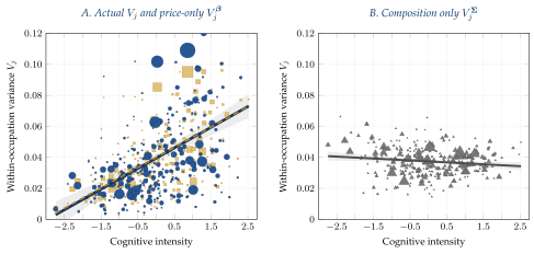
Each point is a three-digit occupation \(j\), plotted against the occupation’s Autor and Dorn (2013) measure of cognitive task intensity. Panel A compares the actual within-occupation variance \(V_{j}\) (blue circles) with the price-only counterfactual \(V_{j}^{\boldsymbol{\beta}}=\boldsymbol{\beta}_{j}'\,\bar{\boldsymbol{\Sigma}}\,\boldsymbol{\beta}_{j}\) (gold squares), which gives each occupation its own vector of skill prices \(\boldsymbol{\beta}_{j}\) but the economy-wide employment-weighted average skill composition \(\bar{\boldsymbol{\Sigma}}\). The two have essentially identical gradients (\(+0.013\)). The actual variance is drawn with a solid line and the price-only counterfactual with a dashed line. Panel B plots the composition-only counterfactual \(V_{j}^{\boldsymbol{\Sigma}} = \bar{\boldsymbol{\beta}}'\,\boldsymbol{\Sigma}_{j}\,\bar{\boldsymbol{\beta}}\) (grey triangles), which gives each occupation its own skill composition \(\boldsymbol{\Sigma}_{j}\) but the economy-wide employment-weighted average vector of skill prices \(\bar{\boldsymbol{\beta}}\). Its gradient is essentially flat (\(-0.001\)). Marker areas are proportional to occupation sample size. For visual clarity the panels are clipped to the employment-weighted 1st–99th percentile of the plotted variables. All outliers are retained in all estimation. ACS 2010 cross-section, \(J = 287\) occupations.