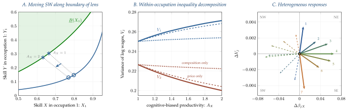
Panel A shows the feasible set \(\mathcal{B}\), with the lower boundary \(\underline{B}(X_1)\) and the contract curve as cognitive productivity \(A_X\) rises from \(1\) to \(2\). Asterisks (\(\boldsymbol{*}\)) mark the bundled equilibrium, open circles (\(\circ\)) mark the unconstrained optimum on the contract curve. Panel B shows the within-occupation variance of log wages \(V_j\) for each occupation, decomposed into a price component (dashed, holding composition fixed) and a composition component (dotted, holding prices fixed). Panel C plots the change in cognitive skill price elasticity \(\Delta\beta_{jX}\) against the change in its within-occupation inequality \(\Delta V_j\) for \(J=7\) occupations, with points numbered and colored from \(j=1\), the most cognitive-intensive, to \(j=7\), the most manual-intensive. Solid arrows show the response to the cognitive productivity shock \(A_X\). Dashed arrows show the mirror-image response to a manual productivity shock \(A_Y\). Parameters: independent Fréchet marginals with \(\theta = 2.25\), CES production with \(\sigma = 0.60\), symmetric economy with \(\eta_1 = \eta_2 = 0.5\) and \(\overline{X}=\overline{Y}\).