1 Introduction
How large are the welfare costs of product market distortions? What kinds of policies can best overcome these distortions? We answer these questions using a dynamic model with heterogeneous firms and endogenously variable markups. In our model, markups distort allocations through three channels. First, the aggregate markup acts like a uniform tax on all firms. Second, there is cross-sectional markup dispersion because larger firms face less competition and so charge higher markups. This markup dispersion gives rise to misallocation of factors of production. Third, there is inefficient entry. Our goal is to quantify these three channels using US micro data and to evaluate policies aimed at reducing the costs of markups.
Our focus in this paper is normative: we quantify the welfare costs of markups through the lens of a dynamic model. But the specific endogenous markup mechanism we study is consistent with key facts stressed in the recent empirical literature. In our model, within a given sector, more productive firms are, in equilibrium, larger and face less elastic demand and so charge higher markups than less productive firms. Shocks that allow more productive firms to grow at the expense of less productive firms will be associated with an increase in the aggregate markup and a decline in the aggregate labor share. In this sense, our model is consistent with the reallocation of production from firms with relatively high measured labor shares to firms with relatively low measured labor shares (Autor et al. 2020; Kehrig and Vincent 2021) and the observation that firms with high markups have been getting larger, driving up the aggregate markup (Baqaee and Farhi 2020).
Our general framework encompasses a range of popular market structures including (i) monopolistic competition with Kimball (1995) demand or symmetric translog demand as in Feenstra (2003), and (ii) oligopolistic competition with nested-CES demand as in Atkeson and Burstein (2008) and Edmond et al. (2015). We consider settings where firms can differ in both productivity and quality and provide aggregation results showing that the macro implications of micro-level markup heterogeneity can be summarized by a few key statistics. One such result is that the aggregate markup, the ‘wedge’ in aggregate employment and investment decisions, is given by the cost-weighted average of firm-level markups.1 By contrast, the empirical literature on the macro implications of markup heterogeneity typically reports the sales-weighted average of firm-level markups.2 We show that the sales-weighted average is the cost-weighted average plus a term reflecting the variance of markups. In this sense the sales-weighted average overstates the aggregate markup by including a term that reflects misallocation rather than the level of markups per se. Importantly, these aggregation results hold independent of the market structure details.
Regardless of market structure, we find that markups distort allocations through the three channels mentioned at the outset: the aggregate markup, misallocation due to markup dispersion, and inefficient entry. We show that the efficient allocation can be implemented by a specific nonlinear schedule of direct subsidies with two components, a uniform component that subsidizes all firms and that can be used to eliminate the aggregate markup, and a size-dependent component that jointly eliminates misallocation and the entry distortion.
We quantify the welfare costs of markups by asking how much the representative consumer would benefit if the economy transitioned from an initial steady state with markup distortions to the efficient steady state. Because eliminating the markup distortions entails a large increase in the capital stock, taking into account the cost of building up the capital stock is critical to correctly assess the welfare gains from such policies. We calibrate the initial steady state using US Census of Manufactures firm-level data from 1972 to 2012 to match levels of sales concentration and the firm-level relationship between markups and market shares observed in 6-digit NAICS sectors, controlling for firm fixed effects and 6-digit NAICS sector-year effects to control for other persistent sources of firm and sector heterogeneity.
Our calibration strategy makes use of the fact that, though the precise mapping depends on market structure, all versions of our model imply a simple firm-level relationship between markups and market shares. We use the estimated parameter values from this relationship to calculate firm-level markups in the model and calculate the welfare costs of these markups. That is, we do not feed into the model separately estimated firm-level markups. We prefer to use the markups implied by our model for two reasons. First, in the Census data we only observe firm-level revenues, not prices and quantities separately. Absent firm-level quantities we cannot disentangle markup levels from output elasticities in production (see Bond et al. 2021; De Ridder et al. 2022, for extensive discussion). Second, we would be cautious to interpret such estimates as ‘true markups’ even if output elasticities were accurately estimated, since such estimates potentially confound the true markup with other distortionary ‘wedges’ — e.g., implicit or explicit input or revenue taxes, factor-adjustment costs, or price rigidities, etc. For these reasons the Census data we use leads a relatively wide range of empirically plausible markup levels. Given this, we report the welfare costs of markups for a wide range of values for the aggregate markup, recalibrating the model each time.
We find that the welfare costs of markups can be large. It turns out that the welfare costs are not just increasing in the level of the aggregate markup we target, they are increasing and convex. Because of this convexity, for some parameterizations of the model we find very large welfare costs of markups, as high as 50% in consumption-equivalent terms. Overall we also find that the costs tend to be lower if we assume monopolistic competition but are much higher if we assume oligopolistic competition.
We then turn to quantifying the relative importance of the three channels by which markups reduce welfare in our model. Across all specifications, we find that the aggregate markup and misallocation channels account for the bulk of the costs of markups and that the entry channel is much less important. That said, the relative importance of the aggregate markup and misallocation channels vary depending on the market structure and target for the aggregate markup. For example, the Kimball specification implies that the share of the total costs accounted for by the aggregate markup increases from 1/2 to 3/4 as we increase the aggregate markup from 1.05 to 1.35. The balance of the costs are almost entirely due to misallocation, the losses from the entry distortion are negligible.
Although the losses from misallocation in our model can be sizeable, accounting for value-added TFP losses of around 2% to 6%, depending on the specification, they are small relative to standard estimates in the literature (Restuccia and Rogerson 2008; Hsieh and Klenow 2009). This is because we measure misallocation using the dispersion in marginal revenue products implied by the endogenous markup distribution in our model, i.e., that relatively small share of the dispersion in marginal revenue products systematically related to market shares. We do not attribute all variation in observed marginal revenue products to markups.
In representative firm models, subsidizing entry (or reducing barriers to entry) so as to increase competition is a powerful tool for reducing the aggregate markup and hence reducing the costs of markups (Bilbiie et al. 2008, 2019). By contrast we find that, with heterogeneous firms, subsidizing entry is not a powerful tool. For all our specifications, we find that even large increases in the number of firms have small effects on the aggregate markup.3 To understand this, recall that the aggregate markup is a cost-weighted average of firm-level markups. An increase in the number of firms has two effects on this weighted average. The direct effect is a reduction in the markup of each firm, due to a reduction in each firm’s market share. But there is also an important compositional effect: small firms face more elastic demand and are more vulnerable to competition from entrants; large firms face less elastic demand and are less vulnerable. So when there is an increase in the number of firms, small, low markup firms contract by more than large, high markup firms and the resulting reallocation keeps the aggregate markup almost unchanged, despite the reduction in firm-level markups. In all our specifications, this offsetting compositional effect is almost as large as the direct effect so overall the aggregate markup falls by a small amount.4
The different specifications we consider each have their own strengths and weaknesses. The model with Kimball demand is more flexible than the model with symmetric translog demand and is better able to match our calibration targets. But the model with translog demand is more tractable than Kimball demand and leads to sharp analytic results. Both monopolistic competition models are simple computationally. The oligopoly model is computationally challenging but has richer empirical content. Though our aggregation results hold regardless of the assumed market structure, the oligopoly model makes a number of predictions that differ from the monopolistic competition models. First, we find larger amounts of markup dispersion and hence larger losses from misallocation in the oligopoly model than in either of the monopolistic competition models. Second, while the monopolistic competition models predict that there are too few firms in equilibrium, the oligopoly model predicts that there are too many. But since the entry margin is not a quantitatively important source of losses in any specification, this qualitative difference is not important.
Existing results on costs of markups. The starting point for discussion of the welfare costs of markups is Dixit and Stiglitz (1977), though the literature goes back to Lerner (1934). Recent work such as Zhelobodko et al. (2012), Dhingra and Morrow (2019) and Behrens et al. (2020) studies variable markups in static models with heterogeneous firms. By contrast, our model is dynamic. Like us, Bilbiie et al. (2008, 2019) study a dynamic model and quantify the costs of markups but they assume a representative firm. We find, however, that firm heterogeneity plays a crucial role in understanding the costs of markups. In our model, markups compensate firms for sunk investments in the creation of a new variety. To the extent that there are positive spillovers from the creation of new varieties, as in the endogenous growth literature, our results may overstate the costs of markups. Atkeson and Burstein (2010, 2019) provide a welfare analysis of innovation policies in firm dynamics models but abstract from variable markups. Peters (2020) studies innovation, firm dynamics, and variable markups but does not evaluate the welfare costs of markups.
Markups and misallocation. In our model markups increase with firm size. This is one form of misallocation in the sense of Restuccia and Rogerson (2008), and Hsieh and Klenow (2009). We find that the gross output productivity losses from this form of misallocation are on the order of 1 to 3%, with value-added productivity losses about double that, on the order of 2 to 6%, reflecting a materials share in gross output just under one-half. We view these numbers as an upper bound on the the gains from size-dependent subsidies since we attribute all of the systematic relationship between firm revenue productivity and firm size to market power, and not to, say, overhead costs as in Autor et al. (2020) and Bartelsman et al. (2013). Because of this we are likely somewhat overstating the true relationship between markups and firm size and overstating the losses from this form of misallocation.
It is important to recognize that we abstract from all other sources of markup variation that may cause misallocation. Firms may operate in different locations or sell different products in different sectors and charge different markups depending on the amount of competition they face in those different markets.5 Policies that condition on location or other relevant market details may be able to address these forms of misallocation too. But implementing finely-tuned policies that condition on details of market conditions location-by-location seems challenging in practice. Given this, we restrict our attention to size-dependent markup variation and we find that the value-added productivity gains from eliminating misallocation due to size-dependent markup variation are likely no more than 2 to 6%.
In related work, (Baqaee and Farhi 2020) calculate that the value-added aggregate productivity gains from eliminating markups are about 20%, much larger than in our model. They find much larger effects because they feed into their calculation all the variation in estimated markups (as in De Loecker et al. 2020; Gutiérrez and Phillippon 2017b) whereas we feed in that component of markups that systematically varies with firm market shares. Because the estimated markups they use are more dispersed than the markups from our model, they find larger effects of markup dispersion on aggregate productivity.
2 Model
There is a representative consumer with preferences over final consumption and labor supply and who owns all the firms. The final good is produced by perfectly competitive firms using inputs from many sectors. Within each sector there are heterogeneous imperfectly competitive firms producing differentiated products using capital, labor and materials. Firms enter by paying a sunk cost in units of labor and then obtain a one-time productivity draw in a randomly allocated sector. Exit is random and there is no aggregate uncertainty. We focus on characterizing the steady state and transitional dynamics after a policy change.
2.1 Setup
A key feature of our analysis is a set of aggregation results that hold regardless of the details of market structure within each sector. We proceed in two steps, first explaining the basic setup and aggregate outcomes that hold independent of market structure within each sector and then turning to the remaining details where market structure matters.
Representative consumer. The representative consumer maximizes \[\tag{1} \sum_{t=0}^{\infty}\beta^t\Big(\log C_{t}-\psi\frac{L_{t}^{1+\nu}}{1+\nu}\Big)\] subject to the budget constraint \[\tag{2} C_t + I_t = W_t L_t + R_t K_t + \Pi_t\] where \(C_t\) denotes consumption of the numeraire final good, \(I_t = K_{t+1}-(1-\delta)K_t\) denotes investment, \(K_t\) denotes physical capital, \(L_t\) denotes labor supply, \(W_t\) the real wage, \(R_t\) the rental rate of capital, and \(\Pi_t\) denotes aggregate profits net of the cost of creating new firms.
The representative consumer’s labor supply satisfies \[\tag{3} \psi C_t L_t^{\nu} = W_t\] and their investment choice satisfies \[\tag{4} 1 = \beta \frac{C_t}{C_{t+1}}(R_{t+1}+1-\delta)\] Since firms are owned by the representative consumer, they use the one-period discount factor \(\beta C_t/C_{t+1}\) to discount future profit flows.
Final good producers. Let \(Y_t\) denote gross output of the final good. This can be used for consumption \(C_t\), investment \(I_t\), or as materials \(X_t\), so that \[\tag{5} C_t + I_t + X_t = Y_t\] The use of the final good as materials gives the model a simple ‘roundabout’ production structure, as in Jones (2011) and Baqaee and Farhi (2020).
The final good \(Y_t\) is produced by perfectly competitive firms using inputs \(y_{t}(s)\) from a continuum of sectors \[\tag{6} Y_t = \left(\int_0^1 y_t(s)^{\frac{\eta-1}{\eta}} \, ds \right)^{\frac{\eta}{\eta-1}}\] where \(\eta>1\) is the elasticity of substitution across sectors \(s\in[0,1]\). Let \(p_t(s)\) denote the price index for sector \(s\). Since the final good is the numeraire, these satisfy \[\tag{7} 1 = \left(\int_0^1 p_t(s)^{1-\eta} \, ds \right)^{\frac{1}{1-\eta}}\]
Within sectors. Within each sector there are imperfectly competitive firms producing differentiated goods. As discussed extensively below, we consider two market structures: monopolistic competition with a continuum of firms \(i\in[0,n_t(s)]\) per sector, or oligopolistic competition with a finite number of firms \(i=1,\dots,n_t(s)\) per sector. Except where noted, our results below hold for both cases.
Technology. Firms enter by paying a sunk cost \(\kappa\) in units of labor and then obtain a one-time productivity draw \(z_i(s) \sim G(z)\) in a random sector \(s\). A firm’s gross output is then \[\tag{8} y_{it}(s) = z_i(s) \left(\phi^{\frac{1}{\theta}}\, v_{it}(s)^{\frac{\theta-1}{\theta}} + (1-\phi)^{\frac{1}{\theta}}\, x_{it}(s)^{\frac{\theta-1}{\theta}} \right)^{\frac{\theta}{\theta-1}}\] where \(v_{it}(s)\) is the firm’s value-added, a composite of physical capital and labor \[\tag{9} v_{it} = k_{it}(s)^{\alpha} l_{it}(s)^{1-\alpha}\] We impose a unit elasticity of substitution between capital and labor. The elasticity of substitution between value-added \(v_{it}(s)\) and materials \(x_{it}(s)\) is given by \(\theta\).
Input demands. Taking input prices as given, cost minimization gives the input demands \[\tag{10} R_t k_{it}(s) = \alpha \left\{\Big(\frac{R_t}{\alpha}\Big)^{\alpha}\Big(\frac{W_t}{1-\alpha}\Big)^{1-\alpha}\right\} v_{it}(s)\] \[\tag{11} W_t l_{it}(s) = (1-\alpha) \left\{\Big(\frac{R_t}{\alpha}\Big)^{\alpha}\Big(\frac{W_t}{1-\alpha}\Big)^{1-\alpha}\right\} v_{it}(s) \\\] where the term in braces on the right is the price index for the value-added composite. In turn, demand for the value-added composite and demand for materials are given by \[\tag{12} v_{it}(s) = \phi \; \Bigg\{\frac{\Big(\frac{R_t}{\alpha}\Big)^{\alpha}\Big(\frac{W_t}{1-\alpha}\Big)^{1-\alpha}}{\Omega_t}\Bigg\}^{-\theta} \; \frac{y_{it}(s)}{z_i(s)}\] and \[\tag{13} x_{it}(s) = (1-\phi) \; \Bigg\{\frac{\; 1 \;}{\Omega_t}\Bigg\}^{-\theta} \; \frac{y_{it}(s)}{z_i(s)}\] where \(\Omega_t\) is the input price index dual to the technologies in (8) and (9), namely \[\tag{14} \Omega_t = \left(\phi\,\left\{ \Big(\frac{R_t}{\alpha}\Big)^{\alpha}\Big(\frac{W_t}{1-\alpha}\Big)^{1-\alpha}\right\}^{1-\theta} + (1-\phi) \right)^{\frac{1}{1-\theta}}\] where materials have a relative price of 1 since they are in units of the numeraire. Notice that the capital/labor and value-added/materials ratios are common to all firms.
Marginal cost. These factor demands imply that a firm’s marginal cost is given by \[\tag{15} \frac{\Omega_t}{z_i(s)}\]
Profits and markups. A firm’s profits are then given by \[\tag{16} \pi_{it}(s) = p_{it}(s)y_{it}(s) - \frac{\Omega_t}{z_i(s)} \, y_{it}(s)\] Firms maximize profits subject to the demand system they face, which depends on the market structure details. At the optimum a firm’s price can be written as a markup \(\mu_{it}(s)\) over marginal cost \[\tag{17} p_{it}(s) = \mu_{it}(s) \, \frac{\Omega_t}{z_i(s)},\qquad \mu_{it}(s)=\frac{\sigma_{it}(s)}{\sigma_{it}(s)-1}\] where \(\sigma_{it}(s)\) denotes the (endogenous) demand elasticity facing firm \(i\). Different demand systems imply different determinants of \(\sigma_{it}(s)\) as discussed below. Profits can then be written in terms of markups and sales \[\tag{18} \pi_{it}(s) = \left(1-\frac{1}{\mu_{it}(s)}\right)\, p_{it}(s) y_{it}(s)\]
Labor shares. Combining a firm’s labor demand from (11)-(12) with markup pricing (17), a firm’s labor share can be written where \(\zeta_t\) denotes the elasticity of output with respect to value-added \[\tag{20} \zeta_t : = \frac{\frac{\phi}{1-\phi}\left\{\Big(\frac{R_t}{\alpha}\Big)^{\alpha}\Big(\frac{W_t}{1-\alpha}\Big)^{1-\alpha}\right\} ^{1-\theta}}{1 \; + \; \frac{\phi}{1-\phi}\left\{\Big(\frac{R_t}{\alpha}\Big)^{\alpha}\Big(\frac{W_t}{1-\alpha}\Big)^{1-\alpha}\right\} ^{1-\theta}}\] This elasticity is common to all firms but in general varies over time. All cross-sectional variation in labor shares is due to cross-sectional variation in markups \(\mu_{it}(s)\).
We next briefly outline how the distribution of markups \(\mu_{it}(s)\) affects productivity within and across sectors. We focus on aggregation results that obtain independent of within-sector market structure.
Aggregate productivity. Let \(k_t(s)\), \(l_t(s)\), and \(x_t(s)\) denote sector-level capital, labor and materials. These are the integrals (or sums) of \(k_{it}(s),l_{it}(s)\) and \(x_{it}(s)\) over \(i\) within \(s\). We can then write the gross output of sector \(s\) as \[\tag{21} y_t(s) = z_t(s) F\,(k_t(s),l_t(s),x_t(s)\,)\] where \[\tag{22} F (k,l,x)= \left(\phi^{\frac{1}{\theta}}\, \Big(k^{\alpha} l^{1-\alpha} \Big)^{\frac{\theta-1}{\theta}} + (1-\phi)^{\frac{1}{\theta}}\, x^{\frac{\theta-1}{\theta}} \right)^{\frac{\theta}{\theta-1}}\] and where sector-level productivity satisfies \[\tag{23} z_t(s) = \left(\int_0^{n_t(s)} \, \frac{q_{it}(s)}{z_i(s)} \, di \right)^{-1}\] where \(q_{it}(s):=y_{it}(s)/y_t(s)\) denotes the relative size of firm \(i\) in sector \(s\). The only difference having a finite number of firms makes is that the integral should be replaced by a finite sum.
Likewise, let \(K_t,\tilde{L}_t\), and \(X_t\) denote aggregate capital, labor used in production, and materials. These are the integrals of \(k_t(s),l_t(s)\) and \(x_t(s)\) over \(s\in[0,1]\). We then have aggregate gross output \(Y_t=Z_t F(K_t,\tilde{L}_t,X_t)\) where aggregate productivity is given in the same way as sector productivity \[\tag{24} Z_t = \left(\int_0^1 \, \frac{q_{t}(s)}{z_t(s)} \, ds \right)^{-1}\] where \(q_t(s):=y_t(s)/Y_t\) denotes the relative size of sector \(s\).
Thus sector-level productivity \(z_t(s)\) is a firm-size-weighted harmonic average of firm-level productivity \(z_i(s)\) and aggregate productivity \(Z_t\) is a sector-size-weighted harmonic average of sector-level productivity. Sector-level productivity and aggregate productivity are affected by markups \(\mu_{it}(s)\) through the effects of markups on the distribution of firm-size \(q_{it}(s)\) within sectors and the distribution of sector-size \(q_t(s)\) across sectors.
Aggregate markup. Let \(\mu_t(s)\) denote the sector-level markup, implicitly defined by the sector-level labor share Combining the sector-level labor share with its firm-level counterpart (19) we can write the sales-share of firm \(i\) in sector \(s\) as \[\tag{26} \frac{p_{it}(s)y_{it}(s)}{p_t (s) y_t(s)} = \frac{\mu_{it}(s)}{\mu_t(s)}\times \frac{l_{it}(s)}{l_t(s)}\] Integrating both sides, the sector-level markup can be written either as an employment-weighted arithmetic average or a sales-weighted harmonic average of firm-level markups, as in (2015), \[\tag{27} \mu_{t}(s) \; = \; \int_0^{n_t(s)} \mu_{it}(s)\; \frac{l_{it}(s)}{l_t(s)} \; di \; = \; \left( \int_0^{n_t(s)} \frac{1}{\mu_{it}(s)} \; \frac{p_{it}(s)y_{it}(s)}{p_t(s)y_t(s)} \; di \right)^{-1}\] where, again, the only difference having a finite number of firms makes is that the integral should be replaced by a finite sum. From either of these and the expression for sector-level productivity \(z_t(s)\) we see that the sector-level markup satisfies \(p_t(s)=\mu_t(s) \Omega_t/z_t(s)\), i.e., the sector price index can be expressed as the sector-level markup over marginal cost.
Likewise, let \(\mathcal{M}_t\) denote the aggregate, economy-wide markup. Following the same steps, this can be written either as an employment-weighted arithmetic average or a sales-weighted harmonic average of sector-level markups \[\tag{28} \mathcal{M}_t \; = \; \int_0^{1} \mu_{t}(s)\; \frac{l_{t}(s)}{\tilde{L}_t} \; ds \; = \; \left( \int_0^1 \frac{1}{\mu_{t}(s)} \; \frac{p_{t}(s)y_{t}(s)}{Y_t} \; ds \right)^{-1}\] The aggregate markup satisfies \(1=\mathcal{M}_t \Omega_t/Z_t\), i.e., the aggregate price level (normalized to one) is the aggregate markup over aggregate marginal cost. We discuss these and related measures of average markups in more detail in Appendix A.
Markup dispersion and productivity. To see how markup dispersion affects productivity, observe from (6) that sector size \(q_t(s)=y_t(s)/Y_t\) satisfies \(q_t(s)=p_t(s)^{-\eta}\) and since \(p_t(s)=\mu_t(s) \Omega_t /z_t(s)\) and \(1=\mathcal{M}_t \Omega_t /Z_t\) we can write \[\tag{29} q_t(s) = \Big(\frac{\mu_t(s)}{\mathcal{M}_t}\; \frac{Z_t}{z_t(s)}\Big)^{-\eta}\] Plugging this into our expressions for aggregate productivity and solving for \(Z_t\) we obtain \[\tag{30} Z_t = \left(\int_0^1 \Big(\frac{\mu_t(s)}{\mathcal{M}_t}\Big)^{-\eta} \; z_t(s)^{\eta-1} \; ds \right)^{\frac{1}{\eta-1}}\] In turn, sector-productivity \(z_t(s)\) and markups \(\mu_t(s)\) depend on the distribution of firm-level productivity \(z_i(s)\) and markups \(\mu_{it}(s)\) within sector \(s\) — but the details of this layer of aggregation do depend on the within-sector market structure.
2.2 Role of Market Structure
In this section we explain how the details of within-sector market structure matter. First, the market structure matters for determining the relative size distribution \(q_{it}(s)=y_{it}(s)/y_t(s)\) within each sector \(s\). That said, taking \(n_t(s)\) as given, we can cover a range of popular specifications in a unified way, as explained below. Second, and more substantively, the market structure matters for the entry problem that determines \(n_t(s)\). The entry problem is simple with monopolistic competition but more involved with oligopolistic competition.6
Relative size distribution. Taking \(n_t(s)\) as given, the relative size distribution \(q_{it}(s)\) within sector \(s\) is pinned down by the static markup-pricing condition (17). To cover alternative specifications in a unified way, we write this as \[\tag{31} f(q) = \frac{\sigma(q)}{\sigma(q)-1} \; \frac{A_t(s)}{z_i(s)},\qquad A_t(s):=\frac{\Omega_t}{p_t(s)d_t(s)}\] where the function \(f(q)\) is proportional to the inverse demand curve, \(\sigma(q)\) is the associated demand elasticity, with markup \(\mu(q)=\sigma(q)/(\sigma(q)-1)\), and where \(p_t(s)\) is the price index for sector \(s\) and \(d_t(s)\) is a demand index that depends on the market structure.7 Let \(q(z\,;A)\) denote the solution to \(p(q)=\mu(q)A/z\) for arbitrary \(A>0\). We then pick the specific value of \(A\) that satisfies the within-sector aggregator. For example:
Monopolistic competition with Kimball demand. Let sector \(s\) consist of a mass \(n_t(s)>0\) firms and let sector output be given implicitly by the Kimball aggregator \[\tag{32} \int_0^{n_t(s)} \Upsilon \Big(\frac{y_{it}(s)}{y_t(s)}\Big)\,di = 1\] where \(\Upsilon(q)\) is strictly increasing and strictly concave. For this specification inverse demand \(f(q)\) and the demand elasticity \(\sigma(q)\) are given by \[\tag{33} f(q) = \Upsilon'(q)\qquad \text{and}\qquad \sigma(q)= -\frac{\Upsilon'(q)}{\Upsilon''(q)q}\] The associated demand index \(d_t(s)\) is given by \[\tag{34} d_t(s) = \left(\int_0^{n_t(s)} \, \Upsilon'(q_{it}(s))q_{it}(s)\, di\right)^{-1}\] The scalar \(A_t(s):=\Omega_t/p_t(s)d_t(s)\) is then pinned down by satisfying the Kimball aggregator and thus depends on the mass of firms \(n_t(s)\).
Oligopolistic competition with CES demand. Let sector \(s\) consist of a finite \(n_t(s)\in\mathbb{N}\) firms and let sector output be given by the CES aggregator \[\tag{35} \sum_{i=1}^{n_t(s)} \Upsilon \Big(\frac{y_{it}(s)}{y_t(s)}\Big) = 1,\qquad \Upsilon(q) = q^{\frac{{\gamma}-1}{\gamma}}\] where \(\gamma>\eta>1\) denotes the elasticity of substitution within sector \(s\). Relative to the Kimball specification we have a finite number of firms, hence genuine strategic interactions, but restrict the kernel of the aggregator \(\Upsilon(q)\) to be a power function. For this specification inverse demand \(f(q)\) is given by \[\tag{36} f(q) = \Upsilon'(q) = \frac{\gamma-1}{\gamma}\, q^{-\frac{1}{\gamma}}\] while the demand index is simply \[\tag{37} d_t(s) = \left(\sum_{i=1}^{n_t(s)} \, \Upsilon'(q_{it}(s))q_{it}(s)\right)^{-1} = \frac{\gamma}{\gamma-1}\] Depending on whether competition is in quantities or prices, the demand elasticity facing a firm of size \(q\) is given by \[\tag{38} \sigma(q) = \left\{\begin{array}{ll} \; \left(\dfrac{1}{\eta}q^{\frac{\gamma-1}{\gamma}} + \dfrac{1}{\gamma}(1-q^{\frac{\gamma-1}{\gamma}})\right)^{-1} \qquad \qquad & \text{[Cournot competition]} \\ & \\ \hspace{1.2em} \eta q^{\frac{\gamma-1}{\gamma}} + \gamma (1-q^{\frac{\gamma-1}{\gamma}}) & \text{[Bertrand competition]} \end{array}\right.\] where \(q^{\frac{\gamma-1}{\gamma}}\) is the sales share of a firm of size \(q\), equal to the kernel of the aggregator \(\Upsilon(q)\) in the CES case but not in general. The scalar \(A_t(s):=\Omega_t/p_t(s)d_t(s)\) is pinned down by satisfying the CES aggregator and thus depends on \(n_t(s)\).
With the relative size distribution \(q_{it}(s)\) solved for in this way, we then know the distribution of markups \(\mu_{it}(s)=\mu(q_{it}(s))\) and hence can compute sector-level productivity \(z_t(s)\) and markups \(\mu_t(s)\) and then aggregate productivity \(Z_t\) and the aggregate markup \(\mathcal{M}_t\).
Entry and exit. Firms enter by paying a sunk cost \(\kappa\) in units of labor and then obtain a one-time productivity draw \(z_i(s)\sim G(z)\) in a randomly allocated sector \(s\in[0,1]\). Let \(N_t = \int_0^1 n_t(s)\,ds\) denote the aggregate mass of firms and let \(M_t=\int_0^1 m_t(s)\,ds\) denote the aggregate mass of entrants. With a continuum of sectors, entry per sector \(m_t(s)\) is IID Poisson with rate parameter \(M_t\).8 Firms operate in their sector, obtaining a stream of profits \(\pi_{it}(s)\), until they are hit with an IID exit shock, which happens with probability \(\varphi\) per period. For each sector \(s\) we then have \[\tag{39} n_{t+1}(s) = (1-\varphi)n_t(s) + m_t(s)\] and hence the aggregate mass of firms evolves according to \(N_{t+1} = (1-\varphi)N_t + M_t\).
Free entry condition. Now consider the decision problem of a potential entrant. In all versions of our model, entry occurs to the point at which ex ante expected discounted profits are offset by the sunk cost \[\tag{40} \kappa W_t \geq \beta \sum_{j=1}^{\infty} (\beta(1-\varphi))^{j-1} \frac{C_t}{C_{t+j}} \, \int_0^1 \bar{\pi}_{t+j}(s) \, ds\] with strict equality whenever \(M_t>0\) and where \(\bar{\pi}_t(s)\) denotes expected profits conditional on operating in sector \(s\). Where these market structures differ is in how these expected profits are calculated. Under monopolistic competition, with a continuum \([0,n_t(s)]\) of firms per sector, the entry of any individual firm \(i\) has no effect on sector-level variables. But under oligopolistic competition, with a finite \(n_t(s)\in\mathbb{N}\) firms per sector, the entry of a new firm has non-negligible effects on post-entry sector-level variables. Specifically:
Monopolistic competition. Let \(\pi_t(z_i,s):=\pi_{it}(s)\) denote the ex post profits of an individual firm with productivity draw \(z_i\) in sector \(s\). In the monopolistic competition case, the expected profits conditional on operating in sector \(s\) are equal to the average profits of the incumbent firms in that sector \[\tag{41} \bar{\pi}_t(s)=\int \pi_t(z_i,s) \, dG(z_i)\]
Oligopolistic competition. Let \(\boldsymbol{z}(s)\) denote a sector-specific vector \[\tag{42} \boldsymbol{z}(s) = (\,z_1(s)\,,\,z_2(s)\,,\,\dots\,,\,z_{n_t(s)}(s)\,)\] of \(n_t(s)\) independent draws from \(G(z)\). Let \(\pi_t(z_i,\boldsymbol{z}(s))\) denote the ex post profits of an individual firm with productivity \(z_i\) in a sector with \(n_t(s)\) other firms with productivities \(\boldsymbol{z}(s)\). The free-entry condition is again given by equation (40) but now the expected profits conditional on operating in sector \(s\) are given by \[\tag{43} \bar{\pi}_t(s) = \iint \pi_{t}(z_i,\boldsymbol{z}(s)) \, dG_{n_{t}(s)}(\boldsymbol{z}(s)) \, dG(z_i)\] where \(G_{n_t(s)}(\boldsymbol{z}(s))=G(z_1)\times G(z_2)\times \cdots \times G(z_{n_t(s)}(s))\) denotes the joint distribution of the vector \(\boldsymbol{z}(s)\). In the oligopolistic competition case, the expected profits from entering sector \(s\) are no longer equal to the average profits of those that do operate in sector \(s\). There are two reasons for this. First, even if firms were identical, an entrant of non-negligible size would reduce the market shares of incumbents, tending to decrease expected profits. Second, sectors are heterogeneous, even two sectors with the same \(n_t(s)\) will have different samples \(\boldsymbol{z}(s)\), and, given this heterogeneity, Jensen’s inequality can push expected profits above average profits.
2.3 Equilibrium
Given an initial mass of firms \(n_0(s)\) per sector and an aggregate capital stock \(K_0\), an equilibrium is (i) a sequence of firm prices \(p_{it}(s)\) and allocations \(y_{it}(s)\), \(k_{it}(s)\), \(l_{it}(s)\), \(x_{it}(s)\) and (ii) aggregate gross output \(Y_t\), consumption \(C_t\), investment \(I_t\), materials \(X_t\), labor \(L_t\), wage rate \(W_t\), rental rate \(R_t\), and mass of entrants \(M_t\) such that firms and consumers optimize and the labor, capital and goods markets all clear. In particular \begin{align} L_t & = \iint l_{it}(s)\, di \,ds + \kappa M_t \\ K_t & = \iint k_{it}(s)\, di \,ds\\ X_t & = \iint x_{it}(s)\, di \,ds \tag{46}\end{align} (or the equivalent finite sums over \(i\) in the case of oligopolistic competition). Note that \(\kappa M_t\) denotes labor used in the entry of new firms.
Solving the model. We discuss the solution method in Appendix D in the supplementary online appendix. The key to solving the model is to recognize that aggregate markups \(\mathcal{M}_t\), aggregate productivity \(Z_t\) and aggregate expected profits \(\bar{\Pi}_t:=\int_0^1 \bar{\pi}_t(s)\,ds\), are given by time-invariant functions of the aggregate mass of firms \(N_t\), independent of all other aggregate variables, say \(\mathcal{M}_t=\mathcal{M}(N_t)\), \(Z_t=Z(N_t)\), and \(\bar{\Pi}_t=\Pi(N_t)\). These functions summarize all the implications of market structure for aggregate outcomes. We solve the model by interpolating these functions and then use the remaining conditions, i.e., the production functions, input choices, optimality conditions of the representative consumer, and our aggregation results to simultaneously determine \(Y_t,C_t,I_t,X_t,L_t,W_t,R_t,M_t\) given the state variables \(N_t\) and \(K_t\).
3 Efficient Allocation
In this section we derive the efficient allocation in our economy by considering the problem of a benevolent planner who faces the same technological and resource constraints as in the decentralized economy. Comparing the efficient allocation chosen by the planner to the decentralized allocation reveals three channels through which markups distort outcomes in the decentralized economy: (i) the aggregate markup acts like a uniform output tax, (ii) markup dispersion gives rise to misallocation of factors of production, and (iii) markups distort the entry margin.
3.1 Planner’s Problem
The planner chooses how many varieties to create, how to allocate inputs, consumption, investment, and employment so as to maximize the representative consumer’s utility taking as given the resource constraints for capital, labor and goods and the production functions for individual varieties. To facilitate comparisons with the decentralized equilibrium, the planner cannot direct the creation of new varieties towards specific sectors. We use asterisks to denote variables in the planner’s problem.
The planner’s problem has two parts: (i) a static allocation problem that determines aggregate productivity, and (ii) a dynamic problem that determines aggregate investment in new varieties, aggregate investment in physical capital, and aggregate employment. The link between the two parts is that the aggregate productivity solving the static allocation problem is a function of the stock of varieties, \(Z_t^*=Z(N_t^*)\), which the planner internalizes when choosing how many varieties to create.
Dynamic problem. Starting with the dynamic problem, just as in the decentralized problem, we can use the resource constraints for capital, labor and goods and the production functions for individual varieties to derive the aggregate production function (22). We can then write the the planner’s problem as maximizing \[\tag{47} \sum_{t=0}^{\infty}\beta^t\Big(\log C^*_{t}-\psi\frac{\big(\tilde{L}^*_t + \kappa (N^*_{t+1}-(1-\varphi)N^*_t)\big)^{1+\nu}}{1+\nu}\Big)\] subject to the resource constraint for goods, \[\tag{48} C^*_t + K^*_{t+1} + X_t^* = Z(N_t^*) F(K_t^*,\tilde{L}^*_t,X_t^*) + (1-\delta)K_t^*\] taking as given the function \(Z(N_t^*)\) implied by the static allocation problem. The initial conditions for this problem are the mass of varieties \(N_0\) and capital stock \(K_0\).
The planner’s optimality conditions for consumption, investment, and employment are standard. The shadow wage is equated to the marginal product of labor \[\tag{49} \psi C_t^* L_t^{*\,\nu}=Z_t^* F_{L,t}^*\] while the marginal product of capital satisfies \[\tag{50} 1 = \beta \frac{C_t^*}{C_{t+1}^*} \Big(\,Z_{t+1}^* F_{K,t+1}^* + 1-\delta \, \Big)\] and the marginal product of materials is simply \(Z_t^* F_{X,t}^*=1\). Comparing these conditions with their decentralized counterparts, we see that the aggregate markup \(\mathcal{M}_t\) acts like a uniform output tax, reducing the overall scale of production and hence reducing the use of all inputs relative to the planner’s problem.
Planner’s choice of varieties. Now consider the planner’s choice of varieties \(N_{t+1}^*\). Letting \(W_t^*=\psi C_t^* L_t^{*\,\nu}\) denote the shadow wage, we can write the first order condition \[\tag{51} \kappa W_t^* = \beta\frac{C_t^*}{C_{t+1}^*}(1-\varphi)\kappa W_{t+1}^* + \beta\frac{C_t^*}{C_{t+1}^*}\, \Big(\frac{d Z_{t+1}^*}{d N_{t+1}^*}\frac{N_{t+1}^*}{Z_{t+1}^*} \Big) \, \frac{Y^*_{t+1}}{N_{t+1}^*}\] Iterating forward this gives \[\tag{52} \kappa W_t^* = \beta \sum_{j=1}^{\infty} (\beta(1-\varphi))^{j-1} \frac{C^*_t}{C^*_{t+j}} \, \Big(\frac{d Z_{t+j}^*}{d N_{t+j}^*}\frac{N_{t+j}^*}{Z_{t+j}^*} \Big) \, \frac{Y^*_{t+j}}{N_{t+j}^*}\] This is the planner’s counterpart to the free-entry condition in the decentralized problem. In the decentralized problem, a firm’s incentive to enter is given by its expected discounted profits, which depend on its markup and sales. By contrast, the planner’s incentive to create new varieties depends on the elasticity of aggregate productivity with respect to the mass of firms — and this depends on the solution to the static allocation problem.
Static allocation problem. Now consider the problem of maximizing aggregate productivity \(Z_t^*\) taking as given \(n_t(s)\). The allocation of activity across sectors \(q_t^*(s)=y_t^*(s)/Y_t^*\) is given by \(q_t^*(s)=(z_t^*(s)/Z_t^*)^{\eta}\) so that in terms of sector-level productivity, aggregate productivity is \(Z_t^*=(\int_0^1 z_t^*(s)^{\eta-1}\,ds)^{1/(\eta-1)}\), i.e., as in (30) but with no dispersion in sector-level markups. In turn, the allocation of activity within sectors \(q_{it}^*(s)=y_{it}^*(s)/y_t^*(s)\) is given by \[\tag{53} \Upsilon'(q_{it}^*(s))d_t^*(s) = \frac{z_t^*(s)}{z_i(s)}\] where \(d_t^*(s)\) is the planner’s demand index, the counterpart of (34) or (37). In other words, at the optimum the planner’s shadow value of a variety is simply the planner’s marginal cost of producing it. This optimality condition holds for both our monopolistic competition model with Kimball demand and our oligopolistic competition model with CES demand. As in the decentralized problem, the scalar \(z_t^*(s)/d_t^*(s)\) is pinned down by satisfying the within-sector aggregator. In our oligopolistic competition model with CES demand this gives sector-level productivity \(z_t^*(s)=(\sum_{i=1}^{n_t(s)} z_{it}^*(s)^{\gamma-1})^{1/(\gamma-1)}\) with constant demand index \(d_t^*(s)=\frac{\gamma}{\gamma-1}\).
There is misallocation in the sense of Hsieh and Klenow (2009) whenever there is variation in marginal revenue products across firms, i.e., when the equilibrium \(q_{it}(s)\) does not coincide with the planner’s \(q_{it}^*(s)\). This happens whenever markups \(\mu_{it}(s)\) vary across firms.
Value of an additional variety. Now consider the value to the planner of an additional variety. Abstracting from any integer constraints on \(n_t(s)\), an application of the envelope theorem gives \[\tag{54} \frac{d Z_t^*}{d n_t(s)}\frac{n_t(s)}{Z_t^*} = \big(d_t^*(s) - 1\big) \, q_t^*(s) \, \frac{Z_t^{*} }{z_t^*(s)}\] To interpret this condition, we use the planner’s demand index to write \[\tag{55} d_t^*(s) - 1 = \int_0^{n_t(s)} \big(\epsilon^*_{it}(s)-1\big)\,p^*_{it}(s)q^*_{it}(s)\, di\] (or the equivalent finite sum in the case of oligopolistic competition), where we define \[\tag{56} \epsilon^*_{it}(s) := \frac{\Upsilon(q^*_{it}(s))}{\Upsilon'(q_{it}^*(s))q_{it}^*(s)}, \qquad \text{and} \qquad p^*_{it}(s) := \Upsilon'(q^*_{it}(s))d_t^*(s)\] The term \(\epsilon^{*}_{it}(s)\) is the inverse elasticity of the within-sector aggregator \(\Upsilon(q)\) evaluated at the planner’s allocation for a particular variety \(q_{it}^*(s)\). The term \(p^*_{it}(s)\) is the social value of an additional unit of that variety, i.e., the planner’s counterpart to the market price.
Comparing the free-entry condition in the decentralized equilibrium to the planner’s entry condition, we recover an important insight of Bilbiie et al. (2008, 2019), Zhelobodko et al. (2012) and Dhingra and Morrow (2019), namely that the planner’s incentives to create new varieties are determined by the inverse elasticity \(\epsilon_{it}^*(s)\) of the aggregator while the incentives for new firms to enter are determined by their markups \(\mu_{it}(s)\). Whether there is too much or too little entry compared to the planner’s allocation is in general ambiguous and depends on precise details of the parameterization.
To summarize, variable markups distort outcomes in the decentralized economy through three channels: (i) the aggregate markup \(\mathcal{M}_t\) acts like a uniform output tax, (ii) markup dispersion \(\mu_{it}(s)\) gives rise to misallocation of factors of production, and (iii) markups distort the entry margin.
4 Quantifying the Model
In this section we outline our parameterization and calibration strategy and our model’s implications for the cross-sectional distribution of markups. We then calculate the aggregate productivity losses due to misallocation.
4.1 Benchmark Parameterization
Kimball demand. To this point we have stressed aggregation results that hold regardless of the details of market structure within each sector. But to quantify the model we need to take a stand on demand and market structure. For our benchmark model we assume monopolistic competition with Kimball demand, as in (32) above. In particular, we assume the Kimball aggregator has the functional form introduced by Klenow and Willis (2016). This specification implies that inverse demand curves are given by9 \[\tag{57} \Upsilon'(q)=\frac{\bar{\sigma}-1}{\bar{\sigma}}\exp\bigg(\frac{1-q^{\,\varepsilon/\bar{\sigma}}}{\varepsilon}\bigg),\qquad \bar{\sigma}>1\] which in turn implies that the demand elasticity \(\sigma(q)\) is log-linear in relative size \[\tag{58} \sigma(q):=-\frac{\Upsilon'(q)}{\Upsilon''(q)q} = \bar{\sigma}\, q^{-\varepsilon/\bar{\sigma}}\] The parameter \(\varepsilon/\bar{\sigma}\) is the elasticity of the demand elasticity with respect to relative size and is often known as the super-elasticity. If \(\varepsilon=0\) we have the constant demand elasticity \(\sigma(q)=\bar{\sigma}\). If \(\varepsilon>0\), relatively large firms will face less elastic demand and charge high markups. If \(\varepsilon<0\), relatively large firms will face more elastic demand and charge low markups.
Productivity distribution. For parsimony and as is standard in the literature we assume that the distribution of productivity \(G(z)\) is Pareto with tail parameter \(\xi\).
Calibration strategy. We assign values to a number of conventional macro parameters that are held constant through all our quantitative exercises. We calibrate the parameters of the demand system and the productivity distribution to match facts on the amount of sales concentration and the relationship between markups and market shares within sectors.10
Assigned parameters. We assume that a period is one year and set the discount factor \(\beta=0.96\) and depreciation rate \(\delta=0.06\). We set the exit rate to \(\varphi=0.04\) to match the employment share of exiting firms, as in Boar and Midrigan (2020). We set the elasticity of value-added to capital \(\alpha=1/3\) and set the elasticity of substitution between value-added and materials to \(\theta=0.5\), both conventional values. Preferences (1) are homothetic and consistent with balanced growth. We set the inverse of the Frisch elasticity of labor supply to \(\nu=1\). We normalize the disutility from labor supply \(\psi\) and the entry cost \(\kappa\) to achieve a steady-state output of \(Y=1\) and a steady-state total mass of firms \(N=1\) for our benchmark economy. We report these parameter choices in Panel A of Table 1.
| Panel A: Assigned Parameters | ||
| \(\beta\) | discount factor | 0.96 |
| \(\delta\) | depreciation rate | 0.06 |
| \(\varphi\) | exit rate | 0.04 |
| \(\alpha\) | elasticity of value-added to capital | 1/3 |
| \(\nu\) | elasticity of labor supply | 1 |
| \(\theta\) | elasticity of substitution between value-added and materials | 0.5 |
| Panel B: Calibrated Parameters | |||||||
| calibration targets | data | ||||||
| \(\mathcal{M}\) | aggregate markup | 1.1 \(\sim\) 1.4 | 1.05 | 1.15 | 1.25 | 1.35 | |
| top 5% sales share | 0.57 | 0.57 | 0.57 | 0.57 | 0.57 | ||
| materials share | 0.45 | 0.45 | 0.45 | 0.45 | 0.45 | ||
| \(\hat{b}\) | regression coefficient | 0.16 | 0.16 | 0.16 | 0.16 | 0.16 | |
| parameter values | |||||||
| \(\xi\) | Pareto tail | 20.70 | 6.84 | 4.07 | 2.89 | ||
| \(\bar{\sigma}\) | demand elasticity | 29.10 | 10.86 | 7.21 | 5.66 | ||
| \(\varepsilon/\bar{\sigma}\) | super-elasticity | 0.16 | 0.16 | 0.16 | 0.16 | ||
| \(\phi\) | weight on value-added | 0.51 | 0.43 | 0.33 | 0.21 | ||
Panel A reports assigned parameters held constant through all our quantitative exercises. Panel B reports calibrated parameters for our benchmark model with monopolistic competition and Kimball demand. We report four cases corresponding to alternative targets for the level of the aggregate markup, \(\mathcal{M}=1.05\), 1.15, 1.25 and 1.35, over the range of \(\mathcal{M}\) implied by the US Census of Manufactures from \(1972\) to \(2012\), as discussed in Appendix B. For each \(\mathcal{M}\) we calibrate the Pareto tail \(\xi\), demand elasticity \(\bar{\sigma}\), super-elasticity \(\varepsilon/\bar{\sigma}\) and weight on value-added \(\phi\) to match the targets shown in Panel B. For each model we choose the super-elasticity \(\varepsilon/\bar{\sigma}\) so that the slope coefficient \(b\) from equation (59) in the model matches the estimated slope coefficient \(\hat{b}\). See the text for more details.
Calibrated parameters. The level and dispersion of markups in our benchmark model depend crucially on three underlying parameters: (i) the Pareto tail parameter \(\xi\), (ii) the super-elasticity \(\varepsilon/\bar{\sigma}\) that determines the sensitivity of a firm’s demand elasticity to its relative size, and (iii) the ‘average’ demand elasticity \(\bar{\sigma}\). Intuitively, the Pareto tail parameter \(\xi\) is pinned down by the amount of concentration in the distribution of firm size, the super-elasticity \(\varepsilon/\bar{\sigma}\) is pinned down by the cross-sectional relationship between markups and market shares, and \(\bar{\sigma}\) is pinned down by the overall level of markups. Specifically we target:
Sales concentration. The Pareto tail parameter \(\xi\) is pinned down by our target for sales concentration. We target the average sales share of the top 5% of firms (by market share) in 6-digit NAICS sectors. For 2012 US manufacturing, the top 5% of firms on average account for 57% of sales.
Relationship between markups and market shares. The super-elasticity \(\varepsilon/\bar{\sigma}\) is pinned down by the relationship between firm-level markups and market shares in our model.11 As discussed in detail below, in our benchmark model the super-elasticity \(\varepsilon/\bar{\sigma}\) corresponds to the slope coefficient \(b\) in a regression of (transformed) markups on market shares. We estimate this regression on firm-level data from the US Census of Manufactures 1972 to 2012 and obtain a precisely estimated \(\hat{b}=0.16\). In our benchmark model this slope coefficient is the super-elasticity so for our benchmark model we set \(\varepsilon/\bar{\sigma}=0.16\). In other versions of our model with different demand systems we use indirect inference, choosing parameters so that the slope coefficient in the model matches the estimated slope coefficient \(\hat{b}=0.16\).
Aggregate Markup. The average elasticity \(\bar{\sigma}\) is pinned down by our target for the aggregate markup \(\mathcal{M}\). As discussed in Appendix B, the aggregate markup we compute in the Census of Manufactures data ranges from about 1.1 to 1.4 depending on the Census year and the specification. The existing literature on markups in the US economy also provides a wide range of estimates for \(\mathcal{M}\).12 Given this range of estimates, rather than commit to a single target for the aggregate markup, for our benchmark model we recalibrate \(\bar{\sigma}\) (jointly, with our other parameters) for \(\mathcal{M}\) ranging from 1.05 to 1.45.
Finally, we calibrate the weight \(\phi\) on value-added in the gross-output production function by targeting a materials share of 45% for the US economy in 2012. For each \(\mathcal{M}\) we calibrate this parameter jointly with the three key parameters \(\xi,\varepsilon/\bar{\sigma}\), and \(\bar{\sigma}\) as discussed above.
Regression specification details. The key to our calibration strategy is the relationship between markups and market shares used to pin down the super-elasticity. To derive this relationship we use the fact that in our model both markups \(\mu_{it}(s)\) and market shares \(\omega_{it}(s)\) are strictly increasing functions of relative size \(q_{it}(s)\). Eliminating \(q_{it}(s)\) we can then write markups as a strictly increasing function of market shares. In particular, as shown in Appendix B, in a version of our model with time-invariant firm-specific demand shifters and sector specific Kimball aggregators, the relationship between market shares and markups works out to be \[\tag{59} \frac{1}{\mu_{it}(s)} + \log\left(1-\frac{1}{\mu_{it}(s)}\right) = a(s) + a_i(s) + a_t(s) + b(s) \, \log \omega_{it}(s),\qquad b(s) = \frac{\varepsilon(s)}{\bar{\sigma}(s)}\] where the firm fixed effects \(a_i(s)\) control for the time-invariant firm-specific demand shifters and the sector-time fixed effects \(a_t(s)\) control for sector-time variation in the Kimball demand index. The transformation on the LHS is strictly increasing in \(\mu_{it}(s)\) and independent of other parameters. In this sense the slope coefficient \(b(s)\) on the RHS is a measure of the strength of the within-sector relationship between markups and market shares. For our benchmark calibration we take the model at face-value and impose a common slope coefficient \(b(s)=b\).13 We estimate this regression using data from the US Census of Manufactures from 1972 to 2012. We construct firm-level markups \(\mu_{it}(s)\) as discussed below and market shares \(\omega_{it}(s)\) within each 6-digit NAICS sector for each Census year. As reported in Table 2, we obtain an estimated slope coefficient \(\hat{b}=0.162\) with standard error 0.002 clustered at the firm level.
Firm-level markups. As discussed in Appendix B, to implement this regression we infer firm-level markups \(\mu_{it}(s)\) from the cost-minimization condition14 \[\tag{60} \mu_{it}(s) = \frac{p_{it}(s)y_{it}(s)}{W_tl_{it}(s)}\times \alpha_t^l(s)\] Our key assumption is that the elasticity of output with respect to labor \(\alpha_t^l(s)\) is common to all firms within a sector.15 Under constant returns to scale,16 we then have, for each firm \[\tag{61} \alpha_t^l(s) = \frac{W_tl_{it}(s)}{W_tl_{it}(s)+R_tk_{it}(s)+x_{it}(s)}\] We estimate this elasticity by averaging (61) over firms within each 6-digit NAICS sector.17 We allow this elasticity to vary over time by constructing it for each Census year. We then have an estimate of \(\alpha_t^l(s)\) that we can plug back into (60) to construct \(\mu_{it}(s)\).
An alternative to this would be to estimate sector-specific production functions. But recent work by Bond et al. (2021) demonstrates that in the presence of variable markups it is not possible to consistently estimate output elasticities when only revenue data is available.18 Using the simple labor input expenditure share approach also makes our results easier to compare to recent empirical work, such as Autor et al. (2020) and De Loecker et al. (2020), that also report such measures.
Other distortions. Our model abstracts from other distortions at either the firm- or sector-level that may drive a wedge between firm revenues and expenditure on labor input. If the relationship between markups and market shares was log-linear, we could use fixed effects to control for persistent firm- or sector-level distortions that confound the measurement of markups in (60). In a robustness exercise, we implement this approach by taking a log-linear approximation to the LHS of (59). See Appendix C in the supplementary online appendix for details.
Model fit. Panel B of Table 1 reports the parameter values that minimize our objective function for four values of the aggregate markup, \(\mathcal{M}=1.05,1.15,1.25\) and \(1.35\). To match a low level of markups, \(\mathcal{M}=1.05\), while targeting a top 5% sales share of 0.57 requires a high average demand elasticity, \(\bar{\sigma}=29.1\), and a thin-tailed productivity distribution, \(\xi=20.7\). To match a high level of markups, \(\mathcal{M}=1.35\), while targeting the same top 5% sales share requires a much lower average demand elasticity, \(\bar{\sigma}=5.66\), and a fatter-tailed productivity distribution \(\xi=2.89\). Though our estimate of \(\varepsilon/\bar{\sigma}=0.162\) is much lower than typically assumed in macro studies that attempt to match the response of prices to changes in monetary policy or exchange rates, it is in line with the micro estimates surveyed by (Klenow and Willis 2016). In Appendix B we find an almost identical super-elasticity \(\varepsilon/\bar{\sigma}=0.16\) best fits the relationship between markups and market shares in the Taiwanese manufacturing firms studied by Edmond et al. (2015).
4.2 Markups and Misallocation
Markup distribution. Table 3 reports the cost-weighted steady-state distribution of markups in our model for the same four values of the aggregate markup. As we target higher levels of the aggregate markup \(\mathcal{M}\) the model implies more markup dispersion. This occurs because as we target higher \(\mathcal{M}\), requiring a lower average demand elasticity \(\bar{\sigma}\), we need a fatter-tailed productivity distribution to hold the top 5% sales share unchanged. In turn, a fatter-tailed productivity distribution creates more large firms who charge large markups, increasing markup dispersion. We illustrate this in Figure 1 using a fine grid for \(\mathcal{M}\).
| cost-weighted distribution of markups | |||||
| aggregate markup, \(\mathcal{M}\) | 1.05 | 1.15 | 1.25 | 1.35 | |
| p25 markup | 1.04 | 1.11 | 1.17 | 1.23 | |
| p50 markup | 1.05 | 1.14 | 1.23 | 1.31 | |
| p75 markup | 1.06 | 1.18 | 1.31 | 1.43 | |
| p90 markup | 1.07 | 1.23 | 1.40 | 1.58 | |
| p99 markup | 1.11 | 1.35 | 1.63 | 1.97 | |
| aggregate productivity losses, % | |||||
| gross output | 0.28 | 0.97 | 1.83 | 2.86 | |
| value-added | 0.61 | 2.71 | 6.08 | 10.73 | |
| value-added, \(\mathcal{M}=1\) | 0.51 | 1.85 | 3.63 | 5.85 | |
Cost-weighted steady-state distribution of markups and aggregate productivity losses for four calibrations of our benchmark model, corresponding to targets for the aggregate markup \(\mathcal{M}=1.05\), 1.15, 1.25 and 1.35. Gross output aggregate productivity loss is \((Z-Z^*)/Z^*\times 100\), and similarly for the value-added aggregate productivity loss. To isolate the effect of misallocation on value-added aggregate productivity we also report the value-added aggregate productivity loss with the same amount of markup dispersion but holding \(\mathcal{M}=1\) to eliminate the distortion between value-added and materials, see text for details.
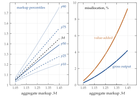
Left panel shows cost-weighted steady-state markup distribution in our benchmark model with monopolistic competition and Kimball demand for a range of targets for the aggregate markup \(\mathcal{M}\). For each \(\mathcal{M}\) we recalibrate the Pareto tail \(\xi\), demand elasticity \(\bar{\sigma}\), super-elasticity \(\varepsilon/\bar{\sigma}\) and weight on value-added \(\phi\) to match the calibration targets in Table 1. Right panel shows implied amounts of misallocation in aggregate gross output and aggregate value-added. To isolate the effect of misallocation on value-added aggregate productivity we report the value-added aggregate productivity loss with the same amount of markup dispersion but holding \(\mathcal{M}=1\) to eliminate the distortion between value-added and materials, see text for details. Shaded interval indicates range of \(\mathcal{M}\) implied by the US Census of Manufactures from \(1972\) to \(2012\), as discussed in Appendix B.
Misallocation. The markup dispersion generated by our model implies that there are aggregate productivity losses due to misallocation. For gross output aggregate productivity we compare \(Z\) in the the steady state of our benchmark economy to the level of gross output aggregate productivity \(Z^*\) that could be achieved by a planner facing the same technology and resource constraints who could reallocate factors of production across producers. As shown in the right panel of Figure 1, for the empirically plausible range of \(\mathcal{M}\), gross output aggregate productivity \(Z\) in our benchmark economy is on the order of 1% to 3% below the level of gross output aggregate productivity \(Z^*\) that could be achieved by a planner.
We also compute value-added aggregate productivity losses. In Appendix G in the supplementary online appendix we show that value-added aggregate productivity can be written \[\tag{62} Z_{\text{value-added}} = \phi^{\frac{1}{\theta-1}}\,\frac{\left(1-\left(1-\phi\right)Z^{\theta-1}\mathcal{M}^{-\theta}\right)}{\left(1-(1-\phi)Z^{\theta-1}\mathcal{M}^{1-\theta}\right)^{\frac{\theta}{\theta-1}}} \, Z\] where \(\phi\) is the weight on value-added, \(\theta\) is the elasticity of substitution between value-added and materials in the gross output production function, and where as above \(Z\) is gross output aggregate productivity. While the level of gross output aggregate productivity \(Z\) is independent of the level of the aggregate markup \(\mathcal{M}\), depending only on markup dispersion, the level of value-added aggregate productivity does depend on the level of \(\mathcal{M}\). This is because the aggregate markup \(\mathcal{M}\) directly distorts the choice of materials relative to value-added.
For the planner, value-added aggregate productivity works out to be \[\tag{63} Z_{\text{value-added}}^* = \phi^{\frac{1}{\theta-1}}\,\frac{\left(1-\left(1-\phi\right)Z^{*\,\theta-1}\right)}{\left(1-(1-\phi)Z^{*\,\theta-1}\right)^{\frac{\theta}{\theta-1}}} \, Z^*\] where \(Z^*\) is the planner’s gross output aggregate productivity. In short, markups reduce value-added aggregate productivity relative to the efficient allocation both because markup dispersion reduces \(Z\) relative to \(Z^*\) and because the aggregate level of markups \(\mathcal{M}\) distorts the use of materials relative to value-added. We report these value-added aggregate productivity losses in Table 3. To isolate the role of markup dispersion we also report the value-added productivity losses that would arise if \(\mathcal{M}=1\), as shown in the right panel of Figure 1.
To illustate the difference in allocations, Figure 2 compares the relative size \(q(z)\) and employment \(l(z)\) of a firm with productivity \(z\) in the decentralized equilibrium to the planner’s counterparts \(q^*(z)\) and \(l^*(z)\). More productive firms have higher markups and produce and employ too little compared to the planner’s allocation. Less productive firms produce and employ too much compared to the planner’s allocation. Notice that the planner’s allocation is not log-linear in productivity, as it would be with CES demand. The extra concavity reflects strongly diminishing marginal productivity as the relative size \(q\) increases. If misallocation losses were calculated assuming a constant demand elasticity \(\bar{\sigma}\) rather than variable demand elasticities \(\sigma(q)=\bar{\sigma}q^{-\varepsilon/\bar{\sigma}}\) we would find higher misallocation (for a given amount of dispersion in marginal revenue products) because we would overstate the gains from reallocating factors from small, less productive firms to large, more productive firms.
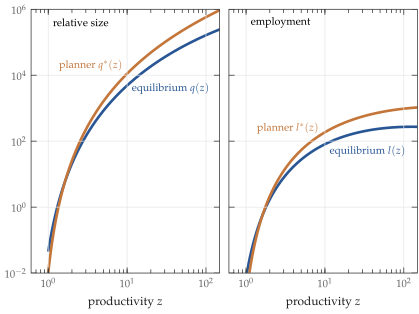
The left panel shows the equilibrium relative size \(q(z)\) and the planner’s relative size \(q^*(z)\) as functions of productivity for our benchmark economy with \(\mathcal{M}=1.15\). The right panel shows the equilibrium employment \(l(z)\) and the planner’s employment \(l^*(z)\) for the same economy. More productive firms have higher markups and produce too little and employ too little compared to the planner’s allocation. Less productive firms produce too much and employ too much compared to the planner’s allocation. In this figure aggregate employment in the decentralized equilibrium is the same as aggregate employment for the planner. Our measure of misallocation is the aggregate output loss implied by the equilibrium allocation relative to the planner’s allocation.
Comparison with Baqaee and Farhi (2020). In related work, (Baqaee and Farhi 2020) calculate that the value-added aggregate productivity gains from eliminating all markups are about 20%, about twice as large as the value-added aggregate productivity gains in even the most extreme calibration of our model. Why do they find much larger effects of markup dispersion on productivity? The key point is that they feed into their calculation all the variation in estimated markups (e.g., as in De Loecker et al. 2020; Gutiérrez and Phillippon 2017b) whereas we feed in that component of markups that systematically varies with firm market shares. In this sense, we use only that part of the cross-sectional variation in markups that is correlated with firm relative size. Because the estimated markups they use are more dispersed than the markups implied by our model, they find larger effects of markup dispersion on aggregate productivity.19
5 How Costly Are Markups?
We now present our main results on the welfare costs of markups. We first quantify the total welfare costs of markups in our benchmark economy for a range of values for the aggregate markup \(\mathcal{M}\). We then show how the efficient allocation can be implemented by a specific nonlinear schedule of size-dependent subsidies and show how to isolate aspects of this policy to quantify the relative magnitudes of the different markup channels. We also study simple entry subsidies that indirectly affect markup distortions through the amount of competition.
We measure the welfare costs of markups by asking how much the representative consumer would benefit from implementing the efficient allocation that eliminates all markup distortions, taking the transitional dynamics into account. We find that the total welfare costs of markups are not only increasing in our target for \(\mathcal{M}\) they are increasing and convex in \(\mathcal{M}\). Because of this, the total welfare costs can be large. For example, for an economy with aggregate markup \(\mathcal{M}=1.15\), implementing the efficient allocation results in a consumption-equivalent welfare gain of about 8.7%, rising to 23.6% for an economy with \(\mathcal{M}=1.25\) and 49.7% for an economy with \(\mathcal{M}=1.35\). We find that a uniform output subsidy that offsets the aggregate markup alone goes a long way towards achieving full efficiency.
5.1 Welfare Cost of Markups
We first compare the distorted steady state in our decentralized equilibrium to that chosen by a planner, then calculate the welfare gains from implementing the efficient steady state taking the transitional dynamics into account.
Steady state comparisons. The first six columns of Table 4 report the percentage change in consumption \(C\), gross output \(Y\), employment \(L\), mass of firms \(N\), physical capital \(K\), and aggregate productivity \(Z\) from the initial distorted steady state to the efficient steady state for each of four values of the aggregate markup \(\mathcal{M}\). The efficient steady state features higher consumption, higher output, and employment. Aggregate productivity is higher, both because of the elimination of misallocation and because of the increase in product variety, i.e., increase in the mass of firms \(N\).20
| steady state comparisons, % | |||||||||
|---|---|---|---|---|---|---|---|---|---|
| \(Y\) | \(C\) | \(L\) | \(N\) | \(K\) | \(Z\) | welfare, % | |||
| \(\mathcal{M}=1.05\) | |||||||||
| efficient | 15.3 | 11.0 | 6.0 | 12.3 | 24.1 | 0.9 | 1.34 | ||
| uniform subsidy | 13.7 | 9.1 | 5.7 | 3.4 | 22.0 | 0.2 | 0.65 | ||
| size-dependent subsidy | 1.4 | 1.7 | 0.3 | 8.1 | 1.7 | 0.7 | 0.71 | ||
| entry subsidy | 1.1 | 1.3 | 0.4 | 11.3 | 1.4 | 0.6 | 0.06 | ||
| \(\mathcal{M}=1.15\) | |||||||||
| efficient | 59.6 | 44.5 | 18.0 | 20.1 | 100.4 | 4.1 | 8.67 | ||
| uniform subsidy | 51.8 | 35.8 | 17.0 | 9.5 | 88.5 | 1.5 | 5.90 | ||
| size-dependent subsidy | 5.3 | 6.2 | 1.0 | 8.3 | 6.6 | 2.3 | 2.87 | ||
| entry subsidy | 6.3 | 7.4 | 2.4 | 20.0 | 8.1 | 3.0 | 0.56 | ||
| \(\mathcal{M}=1.25\) | |||||||||
| efficient | 134.0 | 102.3 | 30.1 | 26.7 | 246.2 | 8.9 | 23.64 | ||
| uniform subsidy | 112.7 | 79.7 | 28.2 | 15.0 | 208.2 | 3.9 | 17.36 | ||
| size-dependent subsidy | 10.8 | 12.5 | 1.8 | 8.1 | 13.6 | 4.1 | 6.26 | ||
| entry subsidy | 17.4 | 20.3 | 6.0 | 29.1 | 23.0 | 7.4 | 1.98 | ||
| \(\mathcal{M}=1.35\) | |||||||||
| efficient | 263.2 | 203.4 | 42.1 | 32.2 | 540.3 | 15.1 | 49.66 | ||
| uniform subsidy | 213.5 | 152.9 | 39.2 | 19.8 | 435.1 | 7.4 | 37.41 | ||
| size-dependent subsidy | 18.4 | 20.9 | 2.7 | 7.6 | 23.6 | 6.0 | 11.32 | ||
| entry subsidy | 38.6 | 44.9 | 11.9 | 39.0 | 52.6 | 14.0 | 5.11 | ||
The first six columns report the percentage change from the initial distorted steady state to the new steady state. The last column reports the consumption equivalent welfare gains (including transitional dynamics). For each \(\mathcal{M}\) we recalibrate the Pareto tail \(\xi\), demand elasticity \(\bar{\sigma}\), super-elasticity \(\varepsilon/\bar{\sigma}\) and weight on value-added \(\phi\). The alternative policies are (i): the efficient allocation, where all markups are removed, (ii) a uniform subsidy that eliminates the aggregate markup, (iii) size-dependent subsidies that eliminate misallocation and the entry distortion, and (iv) the optimal entry subsidy.
Welfare gains from implementing efficient allocation. The last column of Table 4 reports the welfare gains for the representative consumer in consumption-equivalent units including the transition, i.e., these take into account the deferred increase in consumption as investment in physical capital and product variety accumulates over time. These dynamics also take into account the time path of employment. We find that if the aggregate markup is low, \(\mathcal{M}=1.05\), the representative consumer needs to be compensated with an additional 1.34% consumption per period in order to be indifferent between the initial distorted steady state and the transition to the efficient steady state. This increases to 8.67% consumption per period if the aggregate markup is \(\mathcal{M}=1.15\) and to 49.66% consumption per period if the aggregate markup is \(\mathcal{M}=1.35\). The welfare gains are higher when we target higher \(\mathcal{M}\). Indeed the gains are convex in \(\mathcal{M}\). As we target higher \(\mathcal{M}\) for the benchmark economy, both the level of markups and the amount of markup dispersion increase. We illustrate this convexity in Figure 3 using a fine grid for \(\mathcal{M}\) with the upper bound extended to 1.45.
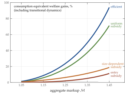
Consumption equivalent welfare gains (including transitional dynamics), from the initial distorted steady state to the new steady state for a range of targets for the aggregate markup \(\mathcal{M}\). For each \(\mathcal{M}\) we recalibrate the Pareto tail \(\xi\), demand elasticity \(\bar{\sigma}\), super-elasticity \(\varepsilon/\bar{\sigma}\) and weight on value-added \(\phi\). The alternative policies are (i): the efficient allocation, where all markups are removed, (ii) a uniform subsidy that eliminates the aggregate markup, (iii) size-dependent subsidies that eliminate misallocation and the entry distortion, and (iv) the uniform entry subsidy that leads to the largest welfare gain. Shaded interval indicates range of \(\mathcal{M}\) implied by the US Census of Manufactures from \(1972\) to \(2012\), as discussed in Appendix B.
5.2 Implementing the Efficient Allocation
We now show how the efficient allocation can be implemented by a specific nonlinear schedule of size-dependent subsidies. This policy removes the aggregate markup distortion, removes markup dispersion (and hence misallocation), and removes the entry distortion. We then show how to isolate different aspects of this policy to quantify the relative magnitudes of the different markup channels. This policy is financed by lump-sum taxes on the representative consumer. We view these calculations as a device for isolating the role of each distortion. The actual consequences of such a policy would of course be much more complex in economies with heterogeneous consumers and other frictions (see Boar and Midrigan 2020, for example).
Direct policy intervention to remove markup distortions. In the decentralized equilibrium, the profits of a firm with productivity \(z\) facing Kimball demand can be written \[\tag{64} \pi_t(z) = \Big[\,\Upsilon'(q_t(z))q_t(z)D_t - \frac{\Omega_t}{z}\, q_t(z) \, \Big]Y_t\] where \(D_t\) denotes the Kimball demand index from (34) above.21 Now suppose that firms are paid a size-dependent subsidy \(T_t(q)\) given by \[\tag{65} T_t(q) = \Big[\,\Upsilon(q)- \Upsilon'(q)q\, \Big] D_t Y_t\] This policy takes away revenues in proportion to \(\Upsilon'(q)q\) and returns revenues in proportion to \(\Upsilon(q)\) which will then induce firms to price at marginal cost. In particular, given the subsidy \(T_t(q)\), a firm has net profits \(\hat{\pi}_t(z):=\pi_t(z)+T_t(q_t(z))\) which simplifies to \[\tag{66} \hat{\pi}_t(z) = \Big[\,\Upsilon(q_t(z))D_t - \frac{\Omega_t}{z}\, q_t(z) \, \Big]Y_t\] This leads to the optimal price \[\tag{67} p_t(z)=\Upsilon'(q_t(z))D_t = \frac{\Omega_t}{z}\] In other words, this policy induces firms to price at marginal cost with firm-level wedge \(\mu_t(z)=1\). Hence the aggregate wedge is also \(\mathcal{M}_t=1\). Given this, net profits are equal to the transfer \(\hat{\pi}_t(z)=T_t(q_t(z))\) and so the free entry condition becomes \begin{align} \tag{68} \kappa W_t & = \beta \sum_{j=1}^{\infty} (\beta(1-\varphi))^{j-1} \frac{C_t}{C_{t+j}} \, \int \Big[\Upsilon(q_{t+j}(z)) - \Upsilon'(q_{t+j}(z))q_{t+j}(z) \Big] D_{t+j} Y_{t+j} \,dG(z) \notag \\ & = \beta \sum_{j=1}^{\infty} (\beta(1-\varphi))^{j-1} \frac{C_t}{C_{t+j}} \, \left(D_{t+j} - 1 \right)\frac{Y_{t+j}}{N_{t+j}} \end{align} where the second line follows using the definitions of the Kimball aggregator (32) and its demand index (34). To see how the free-entry condition under this policy compares to the planner’s entry condition, use (54) to write the planner’s elasticity of aggregate productivity with respect to new varieties \[\tag{69} \frac{d Z_t^*}{d N_t^*}\frac{N_t^*}{Z_t^*} = \left(D_t^* - 1 \right)\] Plugging this elasticity into the planner’s entry condition (52) we see that the free-entry condition under the policy \(T_t(q)\) coincides with the planner’s entry condition, i.e., this policy also eliminates the entry distortion. We next show how to use a generalization of this policy to isolate and quantify the relative importance of each channel.
5.3 Decomposing the Implementation.
The nonlinear schedule \(T_t(q)\) directly implements the efficient allocation. To study each channel in isolation, it is helpful to generalize this to \[\tag{70} T_t(q) = \Big[\, a_0 \,\Upsilon(q) + a_1 \,\Upsilon'(q)q \, \Big] D_t Y_t\] We can then recover the main cases of interest by setting the policy parameters \(a_0,a_1\) appropriately. There are three main cases of interest: (i) setting \(a_0=1\) and \(a_1=-1\) implements the efficient allocation as discussed above, (ii) setting \(a_0=0\) and \(a_1=\chi>0\) implements a uniform subsidy that leaves the dispersion in marginal revenue products unchanged but drives the aggregate wedge down to \(\mathcal{M}/(1+\chi)\), while (iii) setting \(a_0=1/(1+\chi)\) and \(a_1=-1\) implements size-dependent subsidies that eliminate the dispersion in marginal revenue products while leaving an aggregate wedge equal to \(1+\chi\).
Uniform subsidy. Setting \(a_0=0,a_1=\chi\) implements a uniform subsidy giving net profits \[\tag{71} \hat{\pi}_t(z) = \Big[(1+\chi)\Upsilon'(q_t(z))q_t(z)D_t - \frac{\Omega_t}{z}\, q_t(z) \Big]Y_t\] which leads firms to set the price \[\tag{72} p_t(z) = \frac{\mu_t(z)}{1+\chi} \; \frac{\Omega_t}{z}\] where \(\mu_t(z)\) is the benchmark markup of a firm with productivity \(z\). This subsidy induces firms to produce more and to use more of each input, driving the wedge between price and marginal cost down to \(\mu_t(z)/(1+\chi)\) and driving the aggregate wedge in the optimality conditions of the representative firm down to \(\mathcal{M}_t/(1+\chi)\). Thus by setting \(\chi=\mathcal{M}-1\) for the initial distorted steady state we can put in motion a transition to a new steady state where the aggregate wedge has been eliminated. But this uniform subsidy has no effect on relative markups and so leaves steady state misallocation unchanged. This subsidy affects the entry condition but generally leaves it distorted.
Table 4 reports the effect of introducing the uniform subsidy on steady state outcomes for four levels of the aggregate markup \(\mathcal{M}\). Figure 3 reports the effect on welfare, including the transitional dynamics, for a fine grid of \(\mathcal{M}\). For all levels of \(\mathcal{M}\), the uniform subsidy accounts for a large share of the potential welfare gains. For example, if the aggregate markup is low, \(\mathcal{M}=1.05\), the uniform subsidy increases gross output by 13.7%, consumption by 9.1%, and employment by 5.7%. These increases are only slightly smaller than those from implementing the efficient allocation. If the aggregate markup is higher, the uniform subsidy delivers larger increases because the economy is more distorted to begin with. The uniform subsidy delivers less of an increase to aggregate productivity \(Z\) and the mass of firms \(N\) because these reflect the continued presence of misallocation and a distorted entry margin. Notice that as we increase \(\mathcal{M}\), not only are the welfare gains from the uniform subsidy larger, they are also larger as a share of the total gains. For example, if \(\mathcal{M}=1.05\) the uniform subsidy accounts for about one-half of the total welfare gains (0.65% out of 1.34%), rising to nearly three-quarters of the total welfare gains if \(\mathcal{M}=1.35\) (37.41% out of 49.66%).
Size-dependent subsidies. Setting \(a_0=1/(1+\chi)\) and \(a_1=-1\) implements size-dependent subsidies that drives the wedge between price and marginal cost down to \(\mu_t(z)/(1+\chi)=1\) for each firm but leaves the aggregate wedge in the optimality conditions of the representative firm equal to \(1+\chi\). Thus by setting \(\chi=\mathcal{M}-1\) for the initial distorted steady state we can put in motion a transition to a new steady state where the the aggregate wedge remains \(\mathcal{M}\) but where the marginal revenue product of factors are equated across firms, i.e., a new steady state where there is no misallocation, and where the entry distortion is partly offset.
Table 4 shows that such subsidies have a more modest impact than the uniform subsidy. If the aggregate markup is low, \(\mathcal{M}=1.05\), these size-dependent subsidies increase gross output by 1.4%, consumption by 1.7%, and employment by 0.3%, noticeably less than the impact of the uniform subsidy. Where these polices have more success is on aggregate productivity \(Z\) which now increases by 0.7% when misallocation is eliminated as opposed to the 0.2% gain from the uniform subsidy driven by love-of-variety effects. If the aggregate markup is higher, the amount of markup dispersion in the benchmark economy is larger and so the level of misallocation is also higher. In terms of the share of the total gains, the size-dependent subsidies account for about one-half if \(\mathcal{M}=1.05\) (0.71% out of 1.34%), falling to about one-quarter if \(\mathcal{M}=1.35\) (11.32% out of 49.66%).
The direct intervention \(T_t(q)\) eliminates all markup distortions when both the uniform subsidy component and the size-dependent component are switched on. If only one or other of these components is switched on, entry generally remains distorted as well. We next evaluate the extent to which indirect interventions in the product market, such as those which encourage entry and competition, can reduce markup distortions.
5.4 Subsidizing Entry
A policy intervention like \(T_t(q)\) reduces markup distortions directly, i.e., markups act like a tax on production so subsidizing production reduces the distortion. We now contrast such direct policies with a more indirect policy for reducing markup distortions — subsidizing entry, to increase the amount of competition.
Optimal entry subsidy. Consider the introduction of uniform entry subsidy \(\chi_e\) that reduces the sunk entry cost from \(\kappa\) to \(\kappa/(1+\chi_e)\). In Table 4 we report the impact of the optimal entry subsidy that delivers the largest total welfare gain. If the aggregate markup is low, \(\mathcal{M}=1.05\), we find that the optimal entry subsidy delivers a relatively large 11.3% increase in the mass of firms \(N\) but has a more modest effect on economic activity, increasing gross output by 1.1%, consumption by 1.3%, and employment by 0.4%. Aggregate productivity increases by 0.6%, reflecting the increase in variety. But these increases in activity do not lead to substantial welfare gains, due to the cost of creating new varieties incurred during the transition. The gains from the optimal entry subsidy are 0.06%, about one-twentieth of the total gains available (0.06% out of 1.34%). If the aggregate markup is higher, say \(\mathcal{M}=1.15\), the optimal entry subsidy delivers a 20% increase in the mass of firms \(N\) but still entry only accounts for just over one-twentieth of the total gains (0.56% out 8.67%). If \(\mathcal{M}=1.35\), the optimal entry subsidy delivers a 39% increase in the mass of firms \(N\) but still entry accounts for only about one-tenth of the total gains (5.11% out of 49.66%).
Why are the gains from subsidizing entry so low? The gains from entry are low because increasing the number of firms has tiny effects on both the aggregate markup and on misallocation. In this sense, subsidizing entry is too blunt a tool to deal with product market distortions. For example, if the benchmark economy has \(\mathcal{M}=1.05\) the optimal entry subsidy delivers an 11.3% increase in the mass of firms \(N\) but the aggregate markup falls by only about 0.02% to \(\mathcal{M}=1.0498\). Similarly if the benchmark economy has \(\mathcal{M}=1.15\), the optimal entry subsidy delivers a 20% increase in the mass of firms \(N\) but the aggregate markup hardly changes, falling to \(\mathcal{M}=1.149\). Entry subsidies do deliver increases in aggregate productivity, but these are due to love-of-variety effects, not due to a reduction in misallocation.
The result that more competition does not decrease the aggregate markup may appear counterintuitive but is, in fact, a robust result in a large class of models in the international trade literature which have shown that the removal of trade costs (which subjects domestic producers to more competition) leaves the markup distribution unchanged.22 To understand this result, recall that the aggregate markup is a cost-weighted average of firm-level markups. An increase in the number of firms has two effects on this weighted average. The direct effect is a reduction in the relative size \(q\) and hence a reduction in the markups \(\mu(q)\) of each firm. But there is also an important compositional effect. Recall that in our model, small firms face more elastic demand. This makes them more vulnerable to competition from entrants. By contrast large firms face less elastic demand and are less vulnerable to competition from entrants. An entry subsidy that increases the number of firms causes small, low markup firms to contract by more than large, high markup firms and the resulting reallocation means high markup firms get relatively more weight in the aggregate markup calculation. In our model, this offsetting compositional effect is almost exactly as large as the direct effect so that overall the aggregate markup falls by a negligible amount. We develop this argument more formally in Appendix F in the supplementary online appendix.
We illustrate the two offsetting effects in Figure 5. For visual clarity, we consider an extreme parameterization in which we make the entry subsidy large enough to triple the number of firms. Notice in the left panel that markups fall for all firms when the number of firms increases. But the right panel shows that the largest, most productive firms shrink by much less than the smallest, least productive firms. We show below that similar results are obtained with other market structures.
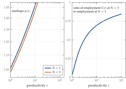
The left panel shows steady-state markups \(\mu(z)\) for an economy with mass of firms \(N=1\) and an entry subsidy chosen to triple the mass of firms to \(N=3\). The right panel shows the ratio of employment \(l(z)\) at \(N=3\) to employment at \(N=1\). Small, low markup firms contract by more than large, high markup firms so that high markup firms get relatively more weight in the aggregate markup calculation. Because of this, the aggregate markup hardly changes. In this example, the aggregate markup barely changes, from \(\mathcal{M}=1.150\) to \(\mathcal{M}=1.146\), even though the mass of firms triples.
5.5 Monopolistic Competition Extensions
We now consider two variations on our benchmark model: (i) where we retain Kimball demand but where firm heterogeneity arises from differences in quality (demand shifters) rather than differences in productivity, and (ii) where we replace Kimball demand with symmetric translog demand. For both these variations we retain the assumption of monopolistic competition. We present results for our model with oligopolistic competition and a finite number of firms per sector in the following section.
5.5.1 Heterogeneity in Quality
In our benchmark model, markups are pinned down entirely by market shares. We now consider an extension where differences in quality imply differences in demand schedules across firms, breaking the tight link between markups and market shares in our benchmark.
Setup. Let \(z\sim G(z)\) denote the quality of a firm’s product and write the Kimball aggregator \[\tag{73} N_t \int \, z \, \Upsilon \Big(\frac{y_{t}(z)}{Y_t}\Big)\,dG(z) = 1\] Following the same steps as in our benchmark model, as shown in Appendix E in the supplementary online appendix, this leads to a relationship between markups and market shares of the form \[\tag{74} \frac{1}{\mu_{t}(z)} + \log\left(1-\frac{1}{\mu_{t}(z)}\right) = a \; + \; b \, \log \omega_t(z) \; - \; b \, \log z, \qquad b =\frac{\varepsilon}{\bar{\sigma}}\] Unlike our benchmark model, cross-sectional variation in market shares is no longer a sufficient statistic for the effect of variation in \(z\). In our benchmark, we interpreted the estimated \(\hat{b}\) as a direct estimate of \(\varepsilon/\bar{\sigma}\). But in this extension, since the market share is negatively correlated with the empirically unobserved quality \(z\), the linear regression coefficient is no longer a consistent estimate of \(\varepsilon/\bar{\sigma}\). In recalibrating the model, we use indirect inference to pin down \(\varepsilon/\bar{\sigma}\), increasing the value of \(\varepsilon/\bar{\sigma}\) until the coefficient in the model \(b\) equals its counterpart in the data, \(\hat{b}=0.162\), jointly with our other calibration targets.
Results. For brevity we focus on the case of \(\mathcal{M}=1.15\). As shown in Appendix E in the supplementary online appendix, the quality model fits the data just as well as our benchmark. The most important difference is that the super-elasticity needs to be substantially higher, \(\varepsilon/\bar{\sigma}=0.304\) as opposed to \(0.162\).23 Given the substantially higher super-elasticity, \(\varepsilon/\bar{\sigma}=0.304\), the quality model implies more markup dispersion, especially in the upper tail. This leads to larger losses from misallocation. Because of this, the total welfare costs are larger than in our benchmark and the gains from size-dependent policies that eliminate misallocation and the entry distortion are both larger in absolute terms and larger as a share of the total than in our benchmark. That said, we continue to find that a uniform output subsidy alone can go more than half way to achieving full efficiency. As in our benchmark, the gains from the optimal entry subsidy are still much smaller than the gains from other policies.
5.5.2 Translog Demand
We now consider a version of our model where we replace Kimball demand with symmetric translog demand as in Feenstra (2003). For this version of the model we revert to our benchmark setting where firm heterogeneity arises from differences in productivity.
Setup. Let the technology for final good producers be given by a symmetric translog expenditure (cost) function which we write \begin{align} \tag{75} \log (P_t Y_t) \; = \; \log Y_t & \; + \; \frac{1}{2 \bar{\sigma} N_t} \; + \; \int \log p_t(z)\,dG(z) \notag \\ & \; + \; \frac{\bar{\sigma} N_t}{2} \, \left(\left(\,\int \log p_t(z)\,dG(z)\right)^2 \, - \, \int \log p_t(z)^{\,2} \,dG(z) \,\right) \end{align}
Markups and market shares. As shown in Appendix E in the supplementary online appendix, the symmetric translog specification implies that the markup \(\mu_t(z)\) of a firm with productivity \(z\) solves the static condition \[\tag{76} \mu + \log \mu = 1 + \log \Big(\frac{z}{z_t^*}\Big),\qquad z>z_t^*\] where \(z_t^*\) is an endogenous productivity cutoff such that firms with \(z<z_t^*\) have zero sales. Moreover the translog specification implies that there is a linear relationship between markups and market shares As in our benchmark model, firms with higher market shares have higher markups. With translog demand, the strength of this relationship is governed by \(1/\bar{\sigma}\). The productivity cutoff \(z_t^*\) is the only aggregate variable that matters for the cross-sectional distribution of markups — and hence the only aggregate variable that matters for the the cross-sectional distributions of market shares \(\omega_t(z)\).
To this point, our characterization of the translog model has restated standard results in the trade literature, familiar from Feenstra (2003), (Rodriguez-Lopez 2011), and (2010, 2019) among others. We next show that given a Pareto distribution of firm-level productivity \(G(z)\) we can solve explicitly for the cutoff productivity \(z_t^*\) and then aggregate markup \(\mathcal{M}_t\). Though closely related to these existing papers, to the best of our knowledge, the following results are novel and may be of some independent interest to researchers working with translog demand and Pareto distributions.
Solving for the cutoff \(z^*_t\). As shown in Appendix F in the supplementary online appendix, the cutoff \(z_t^*\) is given by \[\tag{78} z_t^* = \max \Big[\; 1 \; , \; \bar{\sigma} N_t \,e^{\xi} E_{\xi}(\xi) \; \Big]^{1/\xi}\] where \(E_{n}(x) := \int_1^{\infty} t^{-n} e^{-xt} \,dt\) denotes the generalized exponential integral. Since the mass of firms \(N_t\) is a state variable (is predetermined), this determines \(z_t^*\) and from (76) we then know the entire distribution of markups, market shares and relative prices given \(N_t\). The constant \(e^{\xi} E_{\xi}(\xi)\) depends only on the Pareto tail parameter \(\xi>1\) and is strictly decreasing in \(\xi\), i.e., increasing in productivity dispersion \(1/\xi\). If either the ‘effective’ mass of firms \(\bar{\sigma}N_t\) is sufficiently low or productivity dispersion \(1/\xi\) is sufficiently low we have \(z_t^*=1\), meaning that there are no selection effects and all firms operate. But if either \(\bar{\sigma}N_t\) is sufficiently high or productivity dispersion \(1/\xi\) is sufficiently high we have \(z_t^*>1\), meaning that there are positive selection effects. Intuitively, when demand is more elastic, or when the mass of firms is larger, or when productivity is more dispersed, there is more competitive pressure and selection effects are stronger, increasing the cutoff \(z_t^*\). The right panel of Figure 6 illustrates, showing how the locus \(\bar{\sigma} N_t \,e^{\xi} E_{\xi}(\xi)=1\) partitions the parameter space into the regions where \(z_t^*=1\) (below the curve) and \(z_t^*>1\) (above the curve).
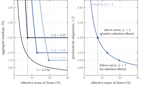
Left panel shows the solution for the aggregate markup \(\mathcal{M}_t\) with translog demand as a function of the effective mass of firms \(\bar{\sigma} N_t\) for various levels of the Pareto tail \(\xi\). Right panel shows how the parameter space is partitioned into regions where there are positive selection effects, \(z_t^*>1\), or no selection effects, \(z_t^*=1\). Whenever there are positive selection effects, the aggregate markup is constant at \(\mathcal{M}_t=1+1/\xi\). By contrast with identical firms, the aggregate markup would be given by \(1+1/\bar{\sigma} N_t\) as shown. With firm heterogeneity, the aggregate markup is decreasing in \(\bar{\sigma} N_t\) only if there are no selection effects, \(z_t^*=1\).
Solving for the aggregate markup \(\mathcal{M}_t\). Our assumption that \(G(z)\) is Pareto also implies a simple solution for \(\mathcal{M}_t\). As shown in Appendix F in the supplementary online appendix, using the fact that the aggregate markup can be written as a harmonic weighted average of firm-level markups, the linear relationship between market shares and markups (77), the static markup condition (76), and our solution for the cutoff productivity \(z_t^*\), the aggregate markup \(\mathcal{M}_t\) is given by \[\tag{79} \mathcal{M}_t = \Big(1+\frac{1}{\xi}\Big) \, \times \, \Big(\max \Big[\; 1 \; , \; \bar{\sigma} N_t \,e^{\xi} E_{\xi}(\xi) \; \Big]\Big)^{-1}\] Since the mass of firms \(N_t\) is a state variable, this determines \(\mathcal{M}_t\). Now observe from (78) that if \(\bar{\sigma} N_t \,e^{\xi} E_{\xi}(\xi)\leq 1\), implying \(z_t^*=1\), then the aggregate markup is strictly decreasing in \(N_t\) with an elasticity of \(-1\). But whenever \(\bar{\sigma} N_t \,e^{\xi} E_{\xi}(\xi)> 1\), i.e., whenever there are positive selection effects, \(z_t^*>1\), then the aggregate markup is constant at the specific value \[\tag{80} \mathcal{M}_t = 1+\frac{1}{\xi},\qquad \text{whenever $z_t^*>1$}\]
So whenever there are positive selection effects, \(z_t^*>1\), e.g., \(\bar{\sigma}\) or productivity dispersion \(1/\xi\) is sufficiently high, then increases in the mass of firms \(N_t\) have no effect on the aggregate markup \(\mathcal{M}_t\). Instead, increases in \(N_t\) are absorbed by increases in the cutoff \(z_t^*\), i.e., by stronger selection effects. This analytic result reinforces the lesson from our benchmark model with Kimball demand where we found numerically that the aggregate markup is extremely insensitive to changes in \(N_t\).24 The reason is the same: whenever \(z_t^*>1\), an increase in \(N_t\) increases \(z_t^*\) thereby directly reducing all firm-level markups \(\mu_t(z)\) according to (76). But low markup firms contract by more than large, high markup firms and the resulting reallocation means high markup firms get relatively more weight in the aggregate markup calculation. In the translog case, so long as parameters are such that \(z_t^*>1\), this offsetting compositional effect is exactly as large as the direct effect so that overall the aggregate markup is unchanged.
Role of heterogeneity. Firm heterogeneity is essential to this result. If by contrast all firms were identical, as in say Bilbiie et al. (2008, 2019), each firm would have market share \(1/N_t\) and the aggregate markup would be \(\mathcal{M}_t=1+1/\bar{\sigma} N_t\) and would always be decreasing in \(N_t\). In the representative firm setting, there is the direct effect of an increase in \(N_t\) on firm-level markups but this effect is the same for all firms so there is no offsetting compositional effect. In this sense, accounting for the role of firm heterogeneity is crucial for understanding the welfare effects of changes in the mass of firms \(N_t\).25
Quantitative results. As discussed in Appendix E in the supplementary online appendix, the translog model does less well in reproducing our calibration targets. As with the quality differences model, the translog model implies considerably more markup dispersion, especially in the upper tail. This leads to larger losses from misallocation relative to our benchmark model. Because of the larger amount of misallocation in the initial distorted steady state, the total welfare costs are larger than in our benchmark and the gains from size-dependent policies that eliminate misallocation and the entry distortion are both larger in absolute terms and larger as a share of the total than in our benchmark. Again we find that the gains from the optimal entry subsidy are much, much smaller than the gains from other policies.
The extensions consider in this section show that, overall, our benchmark results are robust to different monopolistically competitive setups. But one might reasonably suspect that this has more to do with the assumption of monopolistic competition than the specific aggregator we use. Perhaps a fundamentally different market structure will lead to much larger losses from markups? To assess this, we now turn to an alternative model featuring oligopolistic competition with genuine strategic interactions between firms.
6 Oligopolistic Competition
How much does the assumed market structure matter? To assess this, we now present calculations based on an alternative model featuring oligopolistic competition rather than monopolistic competition as used in our benchmark. Our aggregation results hold regardless of the market structure, but we will see that the oligopoly model has richer emprical content and makes a number of predictions that differ from the monopolistic competition benchmark. In particular, we find larger amounts of misallocation and hence larger gains from size-dependent subsidies than in our benchmark model.
Setup. Let there be \(n_t(s)\in\mathbb{N}\) firms per sector with IID productivity draws \(z_i(s)\sim G(z)\). Let the within-sector aggregator be \(\Upsilon(q)=q^{\frac{\gamma-1}{\gamma}}\) for \(\gamma>\eta>1\) so that the model has the nested-CES structure used by Atkeson and Burstein (2008) and Edmond et al. (2015). For our quantitative work we assume Cournot competition so that, as in (38) above, the demand elasticity of a firm is given by the sales-weighted harmonic average \[\tag{81} \sigma_{it}(s) = \left( \, \frac{1}{\eta}\, \omega_{it}(s) \, + \, \frac{1}{\gamma} \, (1-\omega_{it}(s) \, \right)^{-1}\] where \(\omega_{it}(s)=q_{it}(s)^{\frac{\gamma-1}{\gamma}}\) denotes the market share of firm \(i\) in sector \(s\).26 As stressed at length above, this oligopoly model is encompassed by our general framework except that for the free-entry condition (40) expected profits are given by (43). In practice however, solving this oligopoly model with a forward-looking free-entry condition endogenously determining the number of firms is challenging.27 This is because there are many firms that each have non-negligible effects on sector-level outcomes — outcomes in any given sector are a function of the vector \(\boldsymbol{z}(s)= (z_1(s),z_2(s),\dots,z_{n_t(s)}(s))\) of productivities. Because of the finite number of firms, sectors are heterogeneous and we cannot invoke the law of large numbers to compute expected profits. And because \(n_t(s)\) is typically large, we need to compute high-dimensional integrals with respect to the joint distribution \(G_{n_t(s)}(\boldsymbol{z}(s))\) of \(\boldsymbol{z}(s)\). In principle, the heterogeneity across sectors creates incentives for firms to direct entry towards more profitable sectors. But to simplify the problem computationally, we assume that entry is random, that firms can not direct entry in this way. We discuss these issues in more detail in Appendix D in the supplementary online appendix.
Relationship between markups and market shares. This nested-CES specification implies that the inverse markup is linear decreasing in the market share \[\tag{82} \frac{1}{\mu_{it}(s)} = \left(1-\frac{1}{\gamma}\right) - \left(\frac{1}{\eta} - \frac{1}{\gamma} \right) \, \omega_{it}(s)\] As in our benchmark model, firms with higher market shares have higher markups. Here, the strength of this relationship is governed by the gap between the between-sector elasticity of substitution \(\eta\) and the within-sector elasticity of substitution \(\gamma>\eta\). Multiplying both sides of (82) by \(\omega_{it}(s)\) and summing over all firms \(i\) within sector \(s\) gives \[\tag{83} \frac{1}{\mu_{t}(s)} = \left(1-\frac{1}{\gamma}\right) - \left(\frac{1}{\eta} - \frac{1}{\gamma} \right) \, \sum_{i=1}^{n_t(s)} \omega_{it}(s)^2\] The model predicts a linear decreasing relationship between the sector-level inverse markup \(1/\mu_t(s)\) and the sector’s Herfindahl-Hirschman index (HHI) of sales concentration. From (25), the sector-level labor share is proportional to the inverse markup, \(W_t l_t(s)/p_t(s)y_t(s) = (1-\alpha)\zeta_t/\mu_t(s)\). Motivated by this, in calibrating the oligopoly model we use indirect inference to pin down the gap between \(\gamma\) and \(\eta\), choosing parameters so that our model reproduces the \(\hat{b}=-0.21\) slope coefficient in a regression of the change over time of sector-level labor shares on the change in sector-level HHIs, as in Autor et al. (2020), jointly with our other calibration targets.
Calibration. The oligopoly model features both within- and between-sector variation in concentration. We calibrate the oligopoly model targeting measures of concentration within 4-digit sectors in the 2012 US Census of Manufactures as reported by Autor et al. (2020). In particular, we target their top 4 sales share (CR4) of 0.43 and top 20 sales share (CR20) of 0.73. We also target the slope in a regression of the change over time in sector-level labor shares (inverse markups) on the change in sector-level HHIs of \(\hat{b}=-0.21\), i.e., we also target the sectoral relationship between markups and concentration.28 As in our benchmark model we target a materials share of 0.45 and consider a range of targets for the aggrgeate markup \(\mathcal{M}\). Intuitively, the two measures of sales concentration pin down the Pareto tail \(\xi\), which controls the amount of productivity dispersion, and the sunk entry cost \(\kappa\). The aggregate markup then pins down \(\gamma\), while the slope coefficient pins down the gap between \(\gamma\) and \(\eta\). As shown in Table 5, the oligopoly model hits all our calibration targets except when the target for the aggregate markup is low, \(\mathcal{M}=1.05\). For low levels of the aggregate markup, the oligopoly model struggles to reproduce the top 4 sales concentration in the data. For any given \(\mathcal{M}\), the oligopoly model requires less productivity dispersion than the benchmark model with Kimball demand and monopolistic competition. For example, with \(\mathcal{M}=1.15\) the oligopoly model requires Pareto tail \(\xi=8.51\) as opposed to \(\xi=6.84\) in the benchmark model. On average, there is a relatively large number of firms per sector, \(N=359\), but most of these firms are very small.
| calibration targets | data | |||||
| \(\mathcal{M}\) | aggregate markup | 1.1 \(\sim\) 1.4 | 1.05 | 1.15 | 1.25 | 1.35 |
| CR4 | top 4 sales share | 0.43 | 0.37 | 0.43 | 0.43 | 0.43 |
| CR20 | top 20 sales share | 0.72 | 0.76 | 0.72 | 0.72 | 0.72 |
| materials share | 0.45 | 0.45 | 0.45 | 0.45 | 0.45 | |
| \(\hat{b}\) | regression coefficient | −0.21 | −0.21 | −0.21 | −0.21 | −0.21 |
| parameter values | ||||||
| \(\xi\) | Pareto tail | 28.08 | 8.51 | 5.15 | 3.72 | |
| \(\gamma\) | elasticity of substitution within sectors | 59.69 | 12.76 | 7.16 | 5.21 | |
| \(\eta\) | elasticity of substitution between sectors | 1.62 | 1.35 | 1.15 | 0.99 | |
| \(N\) | average number of firms per sector | 415 | 359 | 143 | 112 | |
| \(\phi\) | weight on value-added | 0.70 | 0.58 | 0.46 | 0.30 | |
The calibrated parameters for our oligopoly model. We calibrate the Pareto tail \(\xi\), the within- and between-sector elasticities of substitution \(\gamma\) and \(\eta\), the sunk entry cost \(\kappa\), and weight on value-added \(\phi\) to match the targets shown. In practice, we choose the average number of firms \(N\) per sector and back out the sunk cost \(\kappa\) that rationalizes \(N\). The cross-sectional regression is of the change over time in sector-level labor shares on the change in sector-level HHIs, as discussed in the text. All other parameters are assigned as in Panel A of Table 1.
Results. Table 6 reports the cost-weighted steady-state distribution of firm-level markups \(\mu_{it}(s)\) and sector-level markups \(\mu_t(s)\) for four levels of the aggregate markup \(\mathcal{M}\). The distribution of sector-level markups alone is as dispersed as the unconditional markup distribution in our benchmark model with monopolistic competition calibrated to the same aggregate markup \(\mathcal{M}\) (for which sectors are identical).29 For brevity we focus on the case of \(\mathcal{M}=1.15\). The unconditional distribution of markups in the oligopoly model is considerably more dispersed than in our benchmark, especially in the upper tail. The gross output losses from misallocation are 3.19%, up from 0.97% in the benchmark.
| cost-weighted distribution of markups | ||||||||
| aggregate markup, \(\mathcal{M}\) | 1.05 | 1.15 | 1.25 | 1.35 | ||||
| \(\,\mu_{t}(s)\,\) | \(\,\mu_{it}(s)\,\) | \(\,\mu_{t}(s)\,\) | \(\,\mu_{it}(s)\,\) | \(\,\mu_{t}(s)\,\) | \(\,\mu_{it}(s)\,\) | \(\,\mu_{t}(s)\,\) | \(\,\mu_{it}(s)\,\) | |
| p25 markup | 1.04 | 1.02 | 1.12 | 1.09 | 1.21 | 1.17 | 1.29 | 1.25 |
| p50 markup | 1.05 | 1.04 | 1.14 | 1.11 | 1.23 | 1.19 | 1.32 | 1.27 |
| p75 markup | 1.06 | 1.07 | 1.16 | 1.17 | 1.27 | 1.26 | 1.37 | 1.36 |
| p90 markup | 1.07 | 1.10 | 1.21 | 1.27 | 1.33 | 1.41 | 1.45 | 1.54 |
| p99 markup | 1.11 | 1.20 | 1.35 | 1.57 | 1.57 | 1.90 | 1.78 | 2.24 |
| aggregate productivity losses, % | ||||||||
| gross output | 2.99 | 3.19 | 3.32 | 3.81 | ||||
| value-added | 5.55 | 6.85 | 8.89 | 12.52 | ||||
| value-added, \(\mathcal{M}=1\) | 5.45 | 6.02 | 6.51 | 7.74 | ||||
Cost-weighted steady state distribution of firm-level markups \(\mu_{it}(s)\) and sector-level markups \(\mu_t(s)\) and the implied aggregate productivity losses for our oligopoly model. Gross output aggregate productivity loss is \((Z-Z^*)/Z^*\times 100\), and similarly for the value-added aggregate productivity loss. To isolate the effect of misallocation on value-added aggregate productivity we also report the value-added aggregate productivity loss with the same amount of markup dispersion but holding \(\mathcal{M}=1\) to eliminate the distortion between value-added and materials, see text for details.
As reported in Table 7, in many respects the oligopoly model implies similar long-run changes in economic activity as the benchmark model calibrated to the same \(\mathcal{M}\). For example, for \(\mathcal{M}=1.15\) our benchmark model implies an output increase of 59.6%, consumption increase of 44.5%, and employment increase of 18.0%. For \(\mathcal{M}=1.15\) the oligopoly model implies an output increase of 55.9%, consumption increase of 39.9%, and employment increase of 14.9%. One notable difference however is that in our oligopoly model the initial distorted steady state often features too many firms, for \(\mathcal{M}=1.15\) the efficient steady state involves reducing the average number of firms \(N\) by about 10.5%. In any case, because of the larger amount of misallocation, the oligopoly model implies substantially larger costs of markups, 14.66% in consumption-equivalent terms, up from 8.67% for our benchmark. The gains from size-dependent subsidies that eliminate misallocation and the entry distortion are 8.70% for the oligopoly model, up from 2.87% for our benchmark. The gains from a uniform subsidy that eliminates the aggregate markup distortion are similar to our benchmark, 5.14% down slightly from 5.90%, but are correspondingly a smaller share of the total. Again, the gains from the optimal entry subsidy are much, much smaller than the gains from other policies.30
| steady state comparisons, % | |||||||||
|---|---|---|---|---|---|---|---|---|---|
| \(Y\) | \(C\) | \(L\) | \(N\) | \(K\) | \(Z\) | welfare, % | |||
| oligopoly, \(\mathcal{M}=1.05\) | |||||||||
| efficient | 20.1 | 15.9 | 4.8 | −29.5 | 30.3 | 1.8 | 8.71 | ||
| uniform subsidy | 14.2 | 9.4 | 6.0 | 3.7 | 23.1 | 0.1 | 0.58 | ||
| size-dependent subsidy | 5.3 | 6.1 | −1.1 | −31.4 | 6.1 | 1.7 | 7.97 | ||
| entry subsidy | −2.0 | −2.4 | −1.1 | −28.9 | −2.5 | −1.2 | 0.50 | ||
| oligopoly, \(\mathcal{M}=1.15\) | |||||||||
| efficient | 55.9 | 39.9 | 14.9 | −10.5 | 94.0 | 1.9 | 14.66 | ||
| uniform subsidy | 50.5 | 34.4 | 17.0 | 9.8 | 86.6 | 1.1 | 5.14 | ||
| size-dependent subsidy | 4.1 | 4.4 | −1.8 | −18.4 | 4.5 | 0.8 | 8.70 | ||
| entry subsidy | −2.1 | −2.5 | −1.0 | −8.7 | −2.7 | −1.1 | 0.12 | ||
| oligopoly, \(\mathcal{M}=1.25\) | |||||||||
| efficient | 112.6 | 79.0 | 25.3 | −1.7 | 206.6 | 3.1 | 26.76 | ||
| uniform subsidy | 108.4 | 75.2 | 28.4 | 15.3mn | 201.1 | 3.0 | 15.20 | ||
| size-dependent subsidy | 3.0 | 3.0 | −2.4 | −14.3 | 3.1 | 0.2 | 9.34 | ||
| entry subsidy | 0.9 | 1.0 | 0.4 | 1.9 | 1.2 | 0.4 | 0.01 | ||
| oligopoly, \(\mathcal{M}=1.35\) | |||||||||
| efficient | 204.0 | 142.7 | 35.3 | 3.6 | 412.1 | 5.0 | 48.63 | ||
| uniform subsidy | 201.8 | 141.0 | 39.6 | 20.3 | 411.9 | 5.6 | 32.38 | ||
| size-dependent subsidy | 2.8 | 2.7 | −3.1 | −12.7 | 2.7 | −0.1 | 11.28 | ||
| entry subsidy | 8.3 | 9.4 | 3.4 | 11.1 | 11.2 | 3.2 | 0.44 | ||
The first six columns report the percentage change from the initial distorted steady state with to the new steady state. The last column reports the consumption equivalent welfare gains (including transitional dynamics). The alternative policies are (i): the efficient allocation, where all markups are removed, (ii) a uniform subsidy that eliminates the aggregate markup, (iii) size-dependent subsidies that eliminate misallocation and the entry distortion, and (iv) the optimal entry subsidy (or tax).
There are two important caveats regarding these results. First, in the oligopoly model, subsidies to eliminate misallocation would have to be both sector- and size-dependent, as opposed to just size-dependent as they are in our benchmark model with monopolistic competition. Second, the losses from misallocation may be lower if entry could be directed to specific sectors. It remains an open question and an important direction for future research to assess how much misallocation would be reduced if firms could direct entry.
7 Conclusion
We study the welfare costs of product market distortions in a dynamic model with heterogeneous firms and endogenously variable markups. Our model encompasses several popular market structures and we provide aggregation results showing how the macro implications of micro-level markup heterogeneity can be summarized by a few key statistics. We calibrate our model to match levels of sales concentration and the firm-level relationship between labor shares and market shares observed in 6-digit US Census of Manufactures data. We find that the welfare costs of markups can be large. Depending on the market structure and assumed level of the aggregate markup, the representative consumer can gain as much as 50% in consumption-equivalent terms if all markup distortions are eliminated, once transitional dynamics are taken into account.
In our model markups reduce welfare because the aggregate markup distortion acts like a uniform output tax, reducing employment and investment by all firms, because markup variation across firms causes misallocation of factors of production, and because there is an inefficient rate of entry due to the misalignment between private and social incentives to create new firms. Across all specifications, we robustly find that the aggregate markup and misallocation channels account for the bulk of the costs of markups and that the entry channel is much less important.
Although we focus on the normative side of our model, our results also have clear empirical implications. One simple but important finding is that the overall level of markups is best measured as a cost-weighted average of firm-level markups. This is the relevant ‘wedge’ in aggregate employment and investment decisions. By contrast a sales-weighted average of firm-level markups, as used in the empirical literature, overstates the rise in the overall level of market power. In addition, our results provide two reasons to be skeptical of explanations for the simultaneous rise in concentration and markups that focus on increasing barriers to entry. First, in our model increasing barriers to entry reduce concentration, because the resulting lack of competition makes it easier for small firms to survive. Second, in our model changes in entry have negligible effects on the overall level of markups because entry is associated with a reallocation of production towards high productivity, high markup firms.
To keep our model tractable enough that we can aggregate cross-sectional outcomes and study transitional dynamics for a broad range of alternative market structures, we have abstracted from a number of considerations that might play an important role in the development of a more complete account of the macroeconomic implications of product market distortions. First, while markups in our model are a return to sunk investments, there are no positive spillovers from such investment to the stock of knowledge in the economy at large and hence no implications for endogenous growth. But as emphasized by Atkeson et al. (2019), in the endogenous growth models they survey, a higher markup acts like a uniform subsidy to innovation and is welfare-improving, the quantitative details depending sensitively on the specification of the technology for research. In principle, these effects could be large. That said, in endogenous growth models with variable markups, such as Peters (2020), the interactions between entry, aggregate innovation and misallocation are more subtle with the overall effects on growth ambiguous. An important challenge for future work in this area is to provide detailed evidence on technologies for research and the magnitudes of spillovers that can be used to refine such models to help quantify the relative importance of these growth effects and the level effects of markups emphasized in this paper.
Second, we have made the assumption, standard in the literature, that the underlying sources of firm size differences are fundamental differences in productivity or quality. Because of this, large firms with high markups represent a lost opportunity — they should be even larger, not smaller, but charge lower prices. But if large firms are large not because they are more productive or because their products are higher quality but instead because they receive special tax breaks, or have political connections that help them evade antitrust actions or other forms of regulation, then such firms may well be too large, not too small. Another important challenge for future work in this area is to build models that blend political connections, as in Akcigit et al. (2018), with endogenous product market distortions so that we can quantitatively evaluate size-dependent policy interventions when both fundamental and non-fundamental sources of firm size are operative.
Finally, to keep the analysis focused, we have abstracted from distortionary tax wedges and frictions in factor markets (e.g., monopsony power) that affect aggregate employment and capital accumulation. For standard second best reasons, such distortions may either amplify or mitigate the costs of product market distortions. Quantifying the interactions between these different types of distortions also seems a natural topic for ongoing research.
A Cost-Weighted vs. Sales-Weighted Average Markups
In this appendix we derive an exact relationship between a cost-weighted average markup \(\mathcal{M}\) and a sales-weighted average markup \(\tilde{\mathcal{M}}\). The key result is \[ \boxed{ \, \frac{\tilde{\mathcal{M}}-\mathcal{M}}{\mathcal{M}} = \text{Var}[\hat{\mu}_i] \, }\] where \(\text{Var}[\hat{\mu}_i]\) is a measure of the cross-sectional dispersion in the idiosyncratic component in markups, \(\hat{\mu}_i:=\mu_i/\mathcal{M}\). This derivation makes no assumptions about demand or market structure but makes one key assumption about technology, specifically, that all firms within a given industry have the same cost elasticity.
Notation. Consider an industry with \(i=1,2,\dots,n\) firms. Let \(p_i,y_i,\mu_i\) and \(c_i\) denote respectively a firm’s price, output, markup, and total variable costs.
Cost elasticity assumption. Let \(\vartheta>0\) denote a firm’s cost elasticity, that is, the elasticity of total variable costs with respect to output \[\tag{A1} \vartheta := \frac{\partial \log c}{\partial \log y} = \frac{\partial c}{\partial y} \frac{y}{c} = \frac{\text{marginal cost}}{\text{average cost}}\] Our key assumption is that the cost elasticity \(\vartheta\) is common to all firms within a given industry, \(\vartheta_i=\vartheta\). In other words, all firms within a given industry have the same returns to scale, but this may be either increasing, constant, or decreasing at the industry level. Marginal costs are then given by \(\vartheta c_i/y_i\). Importantly we do not put any restrictions on marginal costs, these can vary arbitrarily across firms within the industry.
Aggregate markup. Given the assumption that all firms within a given industry have the same cost elasticity \(\vartheta\), it is straightforward to show that the industry aggregate markup, that is, the ratio of industry price to industry marginal cost, is given by a cost-weighted average of firm-level markups (equivalently, a sales-weighted harmonic average). Following the same steps as in the main text, since prices \(p_i\) are a markup \(\mu_i\) over marginal cost \(\vartheta c_i/y_i\) we have revenues \(p_i y_i = \vartheta \mu_i c_i\) so if we are to write \(\mathcal{M}\) as the ‘wedge’ between industry revenue \(PY:=\sum_{i} p_i y_i\) and industry costs \(\vartheta \sum_{i} c_i\) (i.e., so that \(\mathcal{M}\) is the ratio of the industry price level to industry marginal costs), then \[\tag{A2} \mathcal{M} = \sum_{i=1}^n \mu_i \, \omega_i,\qquad \omega_i := \frac{c_i}{\sum_{i} c_i}\] where in slight abuse of notation we now use \(\omega_i\) to denote the cost-weights. Notice that this derivation makes no assumptions about the demand system or market structure that generates the markups \(\mu_i\).
Relationship between cost-weighted and sales-weighted averages. By contrast, the applied literature on markups has emphasized sales-weighted averages, which can be written \[\tag{A3} \tilde{\mathcal{M}} = \sum_{i=1}^n \mu_i \, \tilde{\omega}_i,\qquad \tilde{\omega}_i := \frac{p_i y_i}{\sum_{i} p_i y_i}\] We will now show that the sales-weighted average \(\tilde{\mathcal{M}}\) can be decomposed into the cost-weighted average \(\mathcal{M}\) plus a term that reflects the cross-sectional dispersion in markups.
Let \(\mathbb{E}[\cdot]\) denote averages with respect to the cost weights so that \(\mathcal{M} = \mathbb{E}[\mu_i]\). Then we can write the sales-weighted average as \[\tag{A4} \tilde{\mathcal{M}} = \sum_{i=1}^n \mu_i \, \tilde{\omega}_i = \sum_{i=1}^n \mu_i \, \frac{\tilde{\omega}_i}{\omega_i}\, \omega_i = \mathbb{E}\Big[\, \mu_i \, \frac{\tilde{\omega}_i}{\omega_i} \, \Big]\] Expanding the expectation of the product into the covariance plus the product of the expectations then gives \begin{align} \tilde{\mathcal{M}} = \mathbb{E}\Big[\, \mu_i \, \frac{\tilde{\omega}_i}{\omega_i} \, \Big] & = \text{Cov}\Big[\, \mu_i \, , \, \frac{\tilde{\omega}_i}{\omega_i} \, \Big] + \mathbb{E}\big[\mu_i\big] \, \mathbb{E}\Big[\, \frac{\tilde{\omega}_i}{\omega_i} \, \Big] \notag \\ & = \text{Cov}\Big[\, \mu_i \, , \, \frac{\tilde{\omega}_i}{\omega_i} \, \Big] + \mathcal{M} \tag{A5}\end{align} since \(\mathcal{M} = \mathbb{E}[\mu_i]\) and \(\mathbb{E}[\frac{\tilde{\omega}_i}{\omega_i}]=\sum_{i} \tilde{\omega}_i=1\). In short, the absolute difference between the sales-weighted and cost-weighted average markups is given by the covariance of the markups \(\mu_i\) and the relative weights \(\tilde{\omega}_i/\omega_i\).
But under the assumption of a common cost elasticity \(\vartheta\) the relative weights are proportional to the markups themselves \[\tag{A6} \frac{\tilde{\omega}_i}{\omega_i} = \frac{p_i y_i}{c_i} \frac{\sum_{i} c_i}{\sum_{i} p_i y_i} = \frac{\mu_i \vartheta \frac{c_i}{y_i} y_i}{c_i} \frac{\sum_{i} c_i}{\sum_{i} p_i y_i} = \frac{\mu_i}{\mathcal{M}}\] where the last equality follows because \(\mathcal{M}\) is the ‘wedge’ between industry revenue \(\sum_{i} p_i y_i\) and industry costs \(\vartheta \sum_{i} c_i\). In short, we can write \[\tag{A7} \text{Cov}\Big[\, \mu_i \, , \, \frac{\tilde{\omega}_i}{\omega_i} \, \Big] = \text{Cov}\Big[\, \mu_i \, , \, \mu_i \frac{1}{\mathcal{M}} \, \Big] = \frac{1}{\mathcal{M}} \text{Var}[\mu_i]\] And hence our key decomposition can be written \[\tag{A8} \tilde{\mathcal{M}} = \mathcal{M} + \frac{1}{\mathcal{M}} \text{Var}[\mu_i]\] That is, the sales-weighted average can be expressed as the cost-weighted average plus a term that reflects the cross-sectional dispersion in markups.
Multiplicative decomposition. A slightly more intuitive version of this decomposition obtains if we decompose the markups \(\mu_i\) multiplicatively into the common \(\mathcal{M}\) component and an idiosyncratic component \(\hat{\mu}_i\) with mean normalized to one \[\tag{A9} \hat{\mu}_i := \mu_i / \mathcal{M}\] Then \(\text{Var}[\mu_i] = \mathcal{M}^2 \text{Var}[\hat{\mu}_i]\) and we can write \[\tag{A10} \frac{\tilde{\mathcal{M}}-\mathcal{M}}{\mathcal{M}} = \text{Var}[\hat{\mu}_i] \,\] That is, the percentage difference between the sales-weighted average and the cost-weighted average is given by the cross-sectional variance of the idiosyncratic component \(\hat{\mu}_i\).
Hence \(\tilde{\mathcal{M}}\geq \mathcal{M}\) with equality only if there is no markup dispersion. The statistic \(\tilde{\mathcal{M}}\) can rise over time either due to increasing \(\mathcal{M}\) or increasing \(\text{Var}[\hat{\mu}_i]\) or both. The statistic \(\tilde{\mathcal{M}}\) can be rising even if \(\mathcal{M}\) is constant. Indeed \(\tilde{\mathcal{M}}\) can be rising even if \(\mathcal{M}\) is falling if the increase in dispersion \(\text{Var}[\hat{\mu}_i]\) is large enough.
Compustat example. To get a quantitative sense of the difference between the cost-weighted average \(\mathcal{M}\) and the sales-weighted average \(\tilde{\mathcal{M}}\), we compute these statistics using publicly available Compustat data for the US economy. We follow the approach of De Loecker et al. (2020) using the ratio of sales to the cost of goods sold, scaled by estimates (at the 2-digit industry level) of the output elasticity of the production function from (Karabarbounis and Neiman 2019). We show the results in Figure A1.31 Clearly the sales weighted average \(\tilde{\mathcal{M}}\) is higher and has risen by substantially more than the cost-weighted average \(\mathcal{M}\). The additional increase in \(\tilde{\mathcal{M}}\) reflects the increasing dispersion of markups.
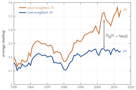
The sales-weighted average \(\tilde{\mathcal{M}}\) of firm-level markups in Compustat data, as in De Loecker et al. (2020), and the cost-weighted average of firm-level markups \(\mathcal{M}\). The former is higher and has increased by a larger amount. The proportional difference between the two averages reflects the cross-sectional dispersion in markups, which has been increasing.
Although researchers may not always have reliable data on total variable costs, under the assumption that all firms within a given industry share the same cost elasticity \(\vartheta\), the cost-weighted arithmetic average is equivalent to the sales-weighted harmonic average, which can of course be computed if the sales-weighted arithmetic average can.
B Census Data and Markup Estimates
We use data from the US Census of Manufactures from 1972 to 2012. We focus on the Census of Manufactures for two reasons: (i) it has higher-quality input data relative to other sectors, such as Services, and (ii) the vast majority of manufacturing goods are easily transportable and not limited to local markets.
Framework. We now spell out the assumptions we need to infer firm-level markups from this Census data. Suppose firms face an inverse demand function and let \(\sigma_{it}(s)\) and \(\mu_{it}(s)\) denote the implied demand elasticity and markup \[\tag{B1} \sigma_{it}(s) := - \frac{\partial \log y_{it}(s)}{\partial \log p_{it}(s)},\qquad \mu_{it}(s):=\frac{\sigma_{it}(s)}{\sigma_{it}(s)-1}\] Suppose firms have production function \[\tag{B2} y_{it}(s) = F_s (k_{it}(s),l_{it}(s),x_{it}(s))\] and let \(\alpha_{it}^k(s),\alpha_{it}^l(s),\alpha_{it}^x(s)\) denote the elasticities of output with respect to capital, labor, and materials \[\tag{B3} \alpha^{k}_{it}(s) := \frac{\partial \log y_{it}(s)}{\partial \log k_{it}(s)},\qquad \alpha^{l}_{it}(s) := \frac{\partial \log y_{it}(s)}{\partial \log l_{it}(s)}, \qquad \alpha^{x}_{it}(s) := \frac{\partial \log y_{it}(s)}{\partial \log x_{it}(s)}\] Taking factor prices as given, suppose \(k_{it}(s),l_{it}(s),x_{it}(s)\) are chosen to maximize profits \[\tag{B4} p_{it}(s)y_{it}(s)-R_t k_{it}(s)-W_t l_{it}(s) - x_{it}(s)\] subject to the inverse demand curve and production function given above. The key first order conditions for this problem can be written \begin{align} R_t k_{it}(s) &= \alpha^k_{it}(s)\frac{p_{it}(s)y_{it}(s)}{\mu_{it}(s)}\\ W_t l_{it}(s) &= \alpha^l_{it}(s)\frac{p_{it}(s)y_{it}(s)}{\mu_{it}(s)}\\ x_{it}(s) &= \alpha^x_{it}(s)\frac{p_{it}(s)y_{it}(s)}{\mu_{it}(s)} \tag{B7}\end{align} which implies, for example,
To infer markups from these conditions using data from the Census of Manufactures we impose two additional assumptions: (i) that each firm \(i\) within a given sector \(s\) has the same factor elasticities, i.e., for each factor \(j=k,l,x\) the elasticities \(\alpha_{it}^j(s)=\alpha_t^j(s)\) for all \(i\) in \(s\), and (ii) the degree of returns to scale in each sector is the same, RTS \(:=\sum_j \alpha_t^j(s)\) for all \(s\). The Census gives us the value of revenue \(p_{it}(s)y_{it}(s)\) and the wage bill \(W_t l_{it}(s)\) for each firm \(i\) in each 6-digit NAICS sector \(s\). Thus if we are equipped with an estimate of the elasticity of output with respect to labor, \(\hat{\alpha}_t^l(s)\) our estimated markups are \[\tag{B9} \hat{\mu}_{it}(s) = \frac{p_{it}(s)y_{it}(s)}{W_t l_{it}(s)} \times \hat{\alpha}_{t}^l (s)\]
Multi-establishment firms. In practice, we begin with the value of shipments \(p_{eit}(s)y_{eit}(s)\) and total salaries/wages \(W_tl_{eit}(s)\) for each establishment \(e\) of firm \(i\) in each 6-digit NAICS sector \(s\). In the case of a single-establishment firm \(i\) in sector \(s\), we have \[\tag{B10} \mu_{it}(s) = \mu_{eit}(s) = \frac{p_{eit}(s)y_{eit}(s)}{W_tl_{eit}(s)}\times \alpha_t^l(s)\] where \(\alpha_t^l(s)\) is the elasticity of output with respect to labor in sector \(s\), as discussed above. For multi-establishment firms we aggregate over the stablishments \(e\) of firm \(i\) to get \[\tag{B11} \mu_{it}(s) = \alpha_t^l(s)\sum_{e\in i} \mu_{eit}(s)\frac{W_t l_{eit}(s)}{\sum_{e'\in i}W_t l_{e'it}(s) }\]
Output elasticities. The empirical literature has proposed various strategies for recovering the output elasticities \(\alpha_t^l(s)\) specific to sector \(s\). In principle, one could estimate sector-specific production functions to recover these elasticities. However, recently Bond et al. (2021) have shown that in the presence of variable markups it is not possible to consistently estimate output elasticities when only revenue data is available. Given this, we follow an alternative approach, more in the spirit of growth accounting, where we use the firm’s cost minimization conditions to write, for each establishment \(e\) and firm \(i\) \[\tag{B12} \alpha_t^l(s) = \frac{W_tl_{eit}(s)}{W_tl_{eit}(s)+R_tk_{eit}(s)+x_{eit}(s)}\times \text{RTS}\] Because of measurement error at the establishment level, we take averages within sector \(s\) for some given RTS. Following Foster et al. (2016), we take the cost-weighted average of labor input expenditure shares of establishments within each sector \(s\). This provides us with an estimate of \(\alpha_t^l(s)\) for each 6-digit NAICS sector \(s\) in each Census year \(t\). For our benchmark results we assume constant returns to scale, RTS \(=1\). We discuss the sensitivity of our results to the RTS in Appendix C in the supplementary online appendix.
Markup regression specification. The key to our calibration of the benchmark model with Kimball demand is the cross-sectional relationship between markups and market shares within a given sector. To see this relationship precisely, consider a version of our model with sector-specific Kimball aggregators with inverse demand curves of the form \[\tag{B13} p_{it}(s) = \Upsilon_s'(q_{it}(s))\gamma_{i}(s)d_t(s),\qquad \Upsilon_s'(q) = \frac{\bar{\sigma}(s)-1}{\bar{\sigma}(s)}\exp\Big(\frac{1-q^{\varepsilon(s)/\bar{\sigma}(s)}}{\varepsilon(s)}\Big)\] where \(d_t(s)\) is the Kimball demand index, common to all firms \(i\) in sector \(s\). Relative to our benchmark model, this more general setting allows for time-invariant firm-specific demand shifters \(\gamma_{i}(s)\) and sector-specific elasticity parameters \(\varepsilon(s),\bar{\sigma}(s)\). Market shares are \(\omega_{it}(s)=p_{it}(s)q_{it}(s)\) so the log market share can be written \[\tag{B14} \log \omega_{it}(s) = \log q_{it}(s) + \frac{1-q_{it}(s)^{\varepsilon(s)/\bar{\sigma}(s)}}{\varepsilon(s)} + \log \Big(\gamma_{i}(s)d_t(s)\frac{\bar{\sigma}(s)-1}{\bar{\sigma}(s)}\Big)\] With Kimball demand the markup \(\mu_{it}(s)\) is related to relative size \(q_{it}(s)\) according to \[\tag{B15} \frac{1}{\mu_{it}(s)} = 1 - \frac{1}{\bar{\sigma}(s)}q_{it}(s)^{\varepsilon(s)/\bar{\sigma}(s)}\] We can then eliminate \(q_{it}(s)\) between equations (B14)-(B15) and collect terms to get \[ \frac{1}{\mu_{it}(s)} + \log \left(1-\frac{1}{\mu_{it}(s)} \right) = a(s) + a_i(s) + a_t(s) + b(s)\log \omega_{it}(s)\] the same as (59) above, with fixed effects \[\tag{B16} a(s) = \frac{\bar{\sigma}(s)-1}{\bar{\sigma}(s)} - \log {\bar{\sigma}(s)} - \frac{\varepsilon(s)}{\bar{\sigma}(s)}\log\Big(\frac{\bar{\sigma}(s)-1}{\bar{\sigma}(s)}\Big)\] \[\tag{B17} a_i(s) = -\frac{\varepsilon(s)}{\bar{\sigma}(s)}\log \gamma_{i}(s)\] \[\tag{B18} a_t(s) = -\frac{\varepsilon(s)}{\bar{\sigma}(s)}\log d_{t}(s)\] and slope coefficient \[\tag{B19} b(s) = \frac{\varepsilon(s)}{\bar{\sigma}(s)}\] To summarize, the model then tells us that the superelasticity is pinned down by the strength of the covariation between (transformed) markups and market shares after having controlled for firm- and sector-time fixed effects. The firm effects control for time-invariant firm-specific demand, \(\gamma_{i}(s)\). The sector-time effects control for sector-specifc implications of shocks that shift the Kimball demand index \(d_t(s)\). For our benchmark specification we take the model at face value and impose a common super-elasticity \(b(s)=b\) for all sectors \(s\). We discuss alternative estimates that relax the assumption of a common super-elasticity and estimate different \(b(s)\) for different subsamples of sectors in Appendix C in the supplementary online appendix.
Outliers. We trim outliers by winsorizing establishment-level markups \(\mu_{eit} (s)\) at the top and bottom \(5\%\) of each Census year.
Interpreting markup estimates. In our view, these markup estimates should be interpreted with some caution, both because of the issue of disentangling markups from output elasticities discussed above and because of the possibility that the firms’ cost-minimization problem is misspecified — in which case, estimated markups will confound true markups with any other distortionary ‘wedge’ between prices and marginal cost, e.g., implicit or explicit input or revenue taxes, factor-adjustment costs, or price rigidities, etc.
Still, if one is prepared to take our estimated firm-level markups from the Census at face value, assuming away any other distortions etc, then one can compute the aggregate markup by taking the appropriate weighted average. We report the results of this exercise in Figure B1. This figure shows the evolution of the aggregate markup (cost-weighted average markup) for two cases, constant returns to scale (RTS \(=1.0\)) and decreasing returns to scale (RTS = \(0.9\)) for each Census year. For RTS \(=1.0\), the aggregate markup ranges from 1.20 in 1972 to a peak of 1.40 in 2002 before declining to about 1.33 in 2012. For RTS = \(0.9\) the aggregate markup is proportionately lower, ranging from 1.08 in 1972, peaking at 1.25 in 2002 before declining to about 1.20 in 2012.
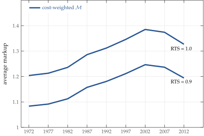
Cost-weighted aggregate markup \(\mathcal{M}\) computed from the firm-level markups \(\mu_{it}(s)\) constructed using micro data from the US Census of Manufactures from \(1972\) to \(2012\), as discussed in the text, for different values of the returns to scale (RTS). Our benchmark model assumes constant returns to scale, RTS \(=1\), but our results are robust to lower returns to scale.
Data Availability
Code replicating the tables and figures in this article can be found in (Edmond et al. 2022) in the Harvard Dataverse, https://doi.org/10.7910/DVN/GVLDPZ.
References
This supplementary appendix is organized as follows. Appendix C provides additional empirical results used to explore the sensitivity of our results to key parameter values. Appendix D explains how we compute the steady state of our model and the transitional dynamics. Appendix E provides further details and quantitative results for two variations on our benchmark model with monopolistic competition: (i) where firm heterogeneity arises from persistence differences in quality across firms, and (ii) where we replace Kimball demand with symmetric translog demand. Appendix F analytically characterizes the aggregate markup with both Kimball demand and symmetric translog demand. These results also give us the mappings \(\mathcal{M}(N)\) and \(Z(N)\) that are crucial ingredients of our computational strategy. Appendix G derives value-added productivity in our model. Appendix H reports a simple formula for the welfare costs of markups in a static version of our model. Finally Appendix I analyzes the ‘love for variety’ effect in our model with Kimball demand.
C Additional Empirical Results
In this appendix we present additional empirical results that explore the sensitivity of our results to key parameter values.
Returns to scale. As discussed in Appendix B in the main text, our estimates of firm-level markups \(\mu_{it}(s)\) require an estimate of the elasticity of output with respect to labor \(\alpha_t^l(s)\). In turn, to estimate this elasticity we need an estimate of the overall returns to scale (RTS) in production, i.e., RTS \(:=\alpha^{k}_t(s)+\alpha^l_{t}(s)+\alpha^x_t(s)\). Given the returns to scale, we can calculate firm-level markups and then estimate the key slope coefficient \(b\) from the within-sector relationship between markups and market shares.
To assess the sensitivity of our results to this assumption, Table C1 reports the estimated slope coefficient \(b=\varepsilon/\bar{\sigma}\) for alternative values of the returns to scale. In particular, if we assume decreasing returns to scale a given input expenditure share implies proportionately lower output elasticities and hence lower levels of the implied markups. If we assume mildly decreasing returns to scale, RTS \(=0.95\) we find that the slope coefficient \(b\) barely changes. It gets slightly larger, rising from our benchmark 0.162 to 0.174, if we assume more strongly decreasing returns to scale, RTS \(=0.90\).
| Dependent Variable | \(\frac{1}{\mu_{it}(s)}+\log\left(1-\frac{1}{\mu_{it}(s)}\right)\) | ||
|---|---|---|---|
| RTS = \(1.00\) | RTS = \(0.95\) | RTS = \(0.90\) | |
| \(\log \omega_{it}(s)\) | 0.162 | 0.162 | 0.174 |
| (0.002) | (0.002) | (0.003) | |
| Sector \(\times\) Year FE | Y | Y | Y |
| Firm FE | Y | Y | Y |
| \(R^2\) | 0.531 | 0.536 | 0.540 |
| Observations | 369,000 | 328,000 | 315,000 |
Sector heterogeneity. Our benchmark calibration takes the model at face-value and imposes a common slope coefficient \(b(s)=b\). To assess the sensitivity of our results to this assumption, we provide alternative estimates of sector-specific \(b(s)\) in two ways.
First, in Table C2 we report estimates of \(b(s)\) with sectors selected by concentration ratios. In particular, we report \(b(s)\) separately for sectors \(s\) with 4-firm concentration ratio (CR4) below and above 40%, a common threshold in the literature. The slope coefficients are very similar across sectors with different concentration levels. Second, in Table C3 we report a full set of \(b(s)\) estimated separately for each 3-digit NAICS sector. For the main specification of interest, with sector \(\times\) year and firm \(\times\) sector fixed effects, we find the slope coefficient \(b(s)\) range from a low of \(b(s)=0.081\) in Wood Product Manufacturing to a high of \(b(s)=0.242\) in Leather and Allied Product Manufacturing. Our benchmark estimate of \(b=0.162\) is almost exactly the midpoint of this range.
| Dependent Variable | \(\frac{1}{\mu_{it}(s)}+\log\left(1-\frac{1}{\mu_{it}(s)}\right)\) | ||
|---|---|---|---|
| Benchmark | CR4 \(>40\%\) | CR4 \(<40\%\) | |
| \(\log \omega_{it}(s)\) | 0.162 | 0.162 | 0.163 |
| (0.002) | (0.009) | (0.002) | |
| Sector \(\times\) Year FE | Y | Y | Y |
| Firm FE | Y | Y | Y |
| \(R^2\) | 0.531 | 0.536 | 0.530 |
| Observations | 369,000 | 21,000 | 348,000 |
| Dependent Variable | \(\frac{1}{\mu_{it}(s)}+\log\left(1-\frac{1}{\mu_{it}(s)}\right)\) | |||||||
|---|---|---|---|---|---|---|---|---|
| \(\log \omega_{it}(s)\) | \(b(s)\) | s.e. | Obs. | \(b(s)\) | s.e. | Obs. | ||
| 311 | Food Manufacturing | 0.058 | 0.002 | 36,500 | 0.179 | 0.009 | 22,000 | |
| 312 | Beverage and Tobacco Product Manufacturing | 0.065 | 0.007 | 4,900 | 0.148 | 0.027 | 3,000 | |
| 313 | Textile Mills | 0.067 | 0.006 | 6,500 | 0.202 | 0.022 | 3,900 | |
| 314 | Textile Product Mills | 0.063 | 0.005 | 11,000 | 0.208 | 0.018 | 6,000 | |
| 315 | Apparel Manufacturing | 0.097 | 0.003 | 31,500 | 0.112 | 0.010 | 12,500 | |
| 316 | Leather and Allied Product Manufacturing | 0.038 | 0.008 | 4,100 | 0.242 | 0.030 | 2,400 | |
| 321 | Wood Product Manufacturing | 0.108 | 0.003 | 31,000 | 0.081 | 0.011 | 19,000 | |
| 322 | Paper Manufacturing | 0.037 | 0.005 | 9,800 | 0.153 | 0.019 | 6,300 | |
| 323 | Printing and Related Support Activities | 0.035 | 0.002 | 71,000 | 0.098 | 0.008 | 4,3000 | |
| 324 | Petroleum and Coal Products Manufacturing | 0.034 | 0.007 | 3,300 | 0.095 | 0.021 | 2,200 | |
| 325 | Chemical Manufacturing | 0.058 | 0.003 | 19,000 | 0.135 | 0.009 | 12,000 | |
| 326 | Plastics and Rubber Products Manufacturing | 0.070 | 0.003 | 27,000 | 0.135 | 0.010 | 17,000 | |
| 327 | Nonmetallic Mineral Product Manufacturing | 0.046 | 0.003 | 32,500 | 0.119 | 0.009 | 22,000 | |
| 331 | Primary Metal Manufacturing | 0.070 | 0.005 | 12,500 | 0.212 | 0.016 | 8,300 | |
| 332 | Fabricated Metal Product Manufacturing | 0.086 | 0.002 | 115,000 | 0.157 | 0.006 | 74,500 | |
| 333 | Machinery Manufacturing | 0.054 | 0.002 | 58,500 | 0.116 | 0.008 | 37,500 | |
| 334 | Computer and Electronic Product Manufacturing | 0.043 | 0.002 | 27,500 | 0.123 | 0.009 | 14,000 | |
| 335 | Electrical Equipment, Appliance, and Component Manufacturing \(\) | 0.055 | 0.004 | 13,000 | 0.154 | 0.014 | 7,900 | |
| 336 | Transportation Equipment Manufacturing | 0.050 | 0.003 | 17,500 | 0.195 | 0.013 | 9,900 | |
| 337 | Furniture and Related Product Manufacturing | 0.075 | 0.003 | 34,000 | 0.166 | 0.012 | 20,000 | |
| 339 | Miscellaneous Manufacturing | 0.054 | 0.002 | 43,500 | 0.166 | 0.009 | 26,500 | |
| Sector \(\times\) Year FE | Y | Y | ||||||
| Firm \(\times\) Sector FE | Y | |||||||
Other distortions and a log-linear specification. Our model implies a non-linear relationship between markups and market size \[ \frac{1}{\mu_{it}(s)} + \log\left(1-\frac{1}{\mu_{it}(s)}\right) = a(s) + a_i(s) + a_t(s) + b(s) \, \log \omega_{it}(s)\] This non-linear relationship makes it difficult to use fixed effects to absorb persistent firm- or sector-level distortions that confound the measurement of markups in (60). To assess the impact of such distortions, we take a log-linear approximation to the LHS to write \[\tag{C1} f(\mu):=\frac{1}{\mu} + \log\left(1-\frac{1}{\mu}\right) \approx f(\bar{\mu}) + f'(\bar{\mu})\bar{\mu} (\log \mu - \log \bar{\mu})\] where \(\bar{\mu}\geq1\) is the point of approximation, a nuisance parameter. Up to this approximation, our model then implies that the true relationship between markups and market size is \[\tag{C2} f(\bar{\mu}) + f'(\bar{\mu})\bar{\mu} (\log \mu_{it}(s) - \log \bar{\mu})= a(s) + a_i(s) + a_t(s) + b(s) \, \log \omega_{it}(s)\] or \[\tag{C3} \log \mu_{it}(s) = \tilde{a} + \tilde{a}(s) + \tilde{a}_i(s) + \tilde{a}_t(s) + \tilde{b}(s) \, \log \omega_{it}(s)\] where \(\tilde{b}(s)=b(s)/(f'(\bar{\mu})\bar{\mu})\) etc where \(f'(\bar{\mu})\bar{\mu}=1/(\bar{\mu}(\bar{\mu}-1))\).
To see the advantage of this log-linear specification, suppose we have measured markups \[\tag{C4} \hat{\mu}_{it}(s) = \frac{p_{it}(s)y_{it}(s)}{W_t l_{it}(s)}\, \hat{\alpha}_t^l(s)\] But suppose the measured markups \(\hat{\mu}_{it}(s)\) confound the true markup \(\mu_{it}(s)\) and a multiplicative wedge \[\tag{C5} \hat{\mu}_{it}(s) = \mu_{it}(s) \exp (\tau_i(s) + \tau_{t}(s))\] Then a regression of log measured markups on log market share is equivalent to \[\tag{C6} \log \hat{\mu}_{it}(s) = \tilde{a} + \tilde{a}(s) + (\tilde{a}_i(s)+\tau_{i}(s)) + (\tilde{a}_t(s)+\tau_t(s)) + \tilde{b}(s) \, \log \omega_{it}(s)\] So the persistent firm-level distortion \(\tau_i(s)\) is absorbed by the firm fixed effects and the persistent sector-time distortion \(\tau_{t}(s)\) is absorbed by the sector-time fixed effects. In this log-linear specification the slope coefficient \(\tilde{b}(s)\) no longer has a structural interpretation, i.e., is not the super-elasticity, but is related to the super-elasticity via \(\tilde{b}(s)=\bar{\mu}(\bar{\mu}-1) b(s)\) where \(\bar{\mu}\geq 1\) is the approximation point.
We report the results from estimating this log-linear specification in Table C4. When we impose a common slope coefficient \(\tilde{b}(s)=\tilde{b}\) as in our benchmark model we find a tightly estimated \(\tilde{b}=0.072\) with standard error 0.001 clustered at the firm level. To intepret this magnitude, if we set \(\bar{\mu}=1.2\) then the implied super-elasticity is \(b=\tilde{b}/(\bar{\mu}(\bar{\mu}-1))=0.072/((1.2)(0.2))=0.3\), somewhat higher than in our benchmark model. That said, this implied value for the super-elasticity is almost exactly the same as the super-elasticity we estimate by indirect inference in an extension of our model where a firm fixed effect is required to control for permanent differences in quality across firms, see Appendix E below.
To summarize, even without imposing the additional structure from the Kimball demand system, we see clearly that markups positively covary with market shares, both within firms over time and across firms at a point in time. Another advantage of this log-linear specification is that the elasticity \(\alpha_t^l(s)\) is also absorbed by the sector-time effects. In this sense, this exercise also serves to demonstrate that our results are not driven by the estimates of \(\alpha_t^l(s)\) used to construct \(\mu_{it}(s)\).
Estimates based on Taiwanese product-level data. As a further robustness check, we have also estimated the slope coefficient \(b\) using a rich product-level panel dataset from Taiwanese manufacturing that we previously studied in Edmond et al. (2015). The Taiwanese data is more detailed than the US Census data and allows us to control for any product-year specific effects. We again construct markups using labor input expenditure shares as in (B10) and estimate the slope coefficient \(b\) in (59) in two ways. In the first approach we exploit the cross-sectional variation of producers within a given product category by including product-year fixed effects. This gives an estimate of \(\hat{b}=0.15\) that is tightly estimated with a standard error of 0.002. In the second approach we exploit the panel structure of the data and include a producer fixed effect, thus using the time-series co-movement of a producer’s sales and their markups to estimate \(b\). This gives an estimate of \(\hat{b}=0.16\) with a standard error of 0.007, almost identical to our benchmark estimate \(\hat{b}=0.162\) from the US Census data.
D Computational Details
In this appendix we outline how we compute the steady state of the model and the transitional dynamics.
D.1 Monopolistic Competition
We first use our aggregation results to calculate the aggregate markup \(\mathcal{M}_{t}\) and aggregate productivity \(Z_{t}\). In our monopolistic competition model, sectors are identical and these are time-invariant functions of the aggregate mass of producers \(N_t\), say \[\tag{D1} \mathcal{M}_{t}=\mathcal{M}(N_t),\qquad \text{and}\qquad Z_t = Z(N_t)\] Calculating these objects requires solving for firm-level markups. To be concrete we illustrate using our Kimball specification. For this specification we can write the problem of a firm with productivity \(z\) as choosing relative output \[\tag{D2} q(z;A) = \operatornamewithlimits{argmax}_{q\geq 0} \; \Big[\, \Upsilon'(q)q-\frac{A}{z}q \,\Big]\] where \(A>0\) is a scalar that summarizes the aggregate conditions faced by an individual firm, including the overall amount of competition, as determined by the demand index \(D\) and the unit cost of production \(\Omega\), as determined by the equilibrium wage and rental rate. Solving this problem for an arbitrary \(A\) gives the relative quantity \(q(z;A)\), which satisfies the complementary slackness condition \[\tag{D3} \Big[\Upsilon'(q(z;A))-\mu(q(z;A))\frac{A}{z}\Big]q(z;A)=0\] where \(\mu(q)=\sigma(q)/(\sigma(q)-1)\) is the markup of a firm of size \(q\) and where for our Kimball specification \(\sigma(q)=\bar{\sigma}q^{-\varepsilon/\bar{\sigma}}\). The equilibrium value of \(A\) is then pinned down by satisfying the Kimball aggregator \[\tag{D4} N\, \int \, \Upsilon(q(z;A)) \, dG(z)=1\] We then have \(A(N)\) for any arbitrary mass of producers \(N>0\). This mapping is time-invariant because the distribution \(G(z)\) is time-invariant.
To implement this, we discretize \(G(z)\) using Gauss-Legendre quadrature with 5000 grid points and obtain \(q(z;A)\) using a non-linear solver for each of these grid points. We then use another non-linear solver to find the equilibrium \(A(N)\) that satisfies the Kimball aggregator. With the optimal relative output \(q(z;A(N))\) and markups \(\mu(q(z;A(N))\) in hand, we can calculate the aggregate markup \(\mathcal{M}(N)\) and aggregate productivity \(Z(N)\) using our aggregation results \[\tag{D5} \mathcal{M}(N) = \left(\dfrac{ \displaystyle{\int} \, \dfrac{1}{\mu(q(z;A(N)))} \, \Upsilon'(q(z;A(N)))q(z;A(N)) \, dG(z)}{\displaystyle{\int} \, \Upsilon'(q(z;A(N)))q(z;A(N)) \, dG(z)} \right)^{-1}\] and \[\tag{D6} Z(N) = \left( N \, \int \, \frac{q(z;A(N))}{z}\, dG(z) \right)^{-1}\]
We interpolate the functions \(\mathcal{M}(N)\) and \(Z(N)\) using Chebyshev polynomials and solve the resulting system of equations that characterize the steady state and transition dynamics using the perfect foresight solver in Dynare. The advantage of the model with monopolistic competition is that the free-entry condition can be written as \[\tag{D7} \kappa W_{t}=\beta\sum_{j=1}^{\infty}(\beta(1-\varphi))^{j-1}\,\frac{C_{t}}{C_{t+j}}\,\left(1-\frac{1}{\mathcal{M}_{t+j}}\right)\,\frac{Y_{t+j}}{N_{t+j}}\] and is therefore straightforward to evaluate alongside the other equilibrium conditions. We use a similar approach to solve for the efficient allocations, replacing the decentralized equilibrium conditions with the first-order conditions that characterize the planner’s allocations.
D.2 Oligopolistic Competition
With oligopolistic competition, the distribution of productivity is no longer sector- and time-invariant. Rather, each sector \(s\) is characterized by a productivity vector \(\boldsymbol{z}(s)=(z_1(s),z_2(s),\dots,z_{n(s)}(s))\) of the \(n(s)\) firms in that sector. Notice here that \(\boldsymbol{z}(s)\) varies across sectors both because the number of firms varies and because, with a finite number of firms, the exact configuration of productivity draws also varies even for two sectors with the same number of firms.
Let \(\lambda(\boldsymbol{z})\) denote the distribution of productivity vectors \(\boldsymbol{z}\) across sectors. For a given \(\lambda(\boldsymbol{z})\), we can solve for the aggregate markup and aggregate productivity by first calculating the within-industry equilibrium for each \(\boldsymbol{z}\). For example, when firms compete in quantities, we solve the following system of \(2n(s)\) equations \[\tag{D8} \mu(z_i,s)= \frac{1}{1-\left(\frac{1}{\eta}\omega(z_i,z)+\frac{1}{\gamma}(1-\omega(z_i,s))\right)}\] \[\tag{D9} \omega(z_i,s) = \frac{\mu(z_i,s)^{1-\gamma} \, z_i^{\gamma-1}}{\displaystyle{\sum}_{i=1}^{n(s)}\, \mu(z_i,s)^{1-\gamma} \, z_i^{\gamma-1}}\] for each firm \(i=1,2,\dots,n(s)\) in each sector \(s\). We can then use the resulting distribution of markups and relative size within and across sectors and the aggregation results in the main text to calculate the aggregate markup and aggregate productivity. Our assumption that entry is random, not directed at individual sectors, allows us to write these aggregate variables as functions of the average number of firms per sector, \(N=\int_0^1 n(s)\, ds\), just as in the model with monopolistic competition.
Now consider the free-entry condition. To evaluate this condition, we need to recognize that a potential entrant understands that, because there are a finite number of firms, its entry will change the equilibrium in the sector it enters. If an entrant is assigned to sector \(s\) with existing productivity distribution \(\boldsymbol{z}(s)=(z_1(s),z_2(s),\dots,z_{n(s)}(s))\) the entrant understands that the configuration of productivity will become \[\tag{D10} \boldsymbol{z}'(s)=(\boldsymbol{z}(s),z)\] where \(z\) is the entrant’s productivity, independently drawn from \(G(z)\).
To implement this, we solve for the industry equilibrium for every sector and every possible draw of \(z\). In practice we have more than 300 firms per sector, it infeasible to use tensor-based Gaussian quadrature to approximate the distribution \(\lambda(\boldsymbol{z})\) across sectors. Instead, we use Monte-Carlo methods to approximate \(\lambda(\boldsymbol{z})\) across 100,000 sectors (we also verify that our answers do not change when we increase the number of sectors further). We again use Gauss-Legendre quadrature to approximate the univariate distribution \(G(z)\).
Let \(\hat{\Pi}(N)\) denote a firm’s expected profits per period (scaled by aggregate output) from entering and drawing productivity \(z\) from \(G(z)\) and being assigned to a random sector \(s\) with initial productivity configuration \(\boldsymbol{z}(s)\), that is \[\tag{D11} \hat{\Pi}(N) = \int \left(\int_0^1 \left(1-\frac{1}{\mu(z,(\boldsymbol{z}(s),z))}\right)\, \omega(z,(\boldsymbol{z}(s),z)) \, \bar{\omega}(\boldsymbol{z}(s),z) \, ds \right) \, dG(z)\] where \(\mu(z,(\boldsymbol{z}(s),z))\) and \(\omega(z,(\boldsymbol{z}(s),z))\) denote the markup and market share of an individual firm with productivity \(z\) in a sector with productivity configuration \(\boldsymbol{z}'(s)=(\boldsymbol{z}(s),z)\) and where \(\bar{\omega}(\boldsymbol{z}(s),z)\) denotes the associated market share of sector \(s\) to which the firm is assigned. Because firms are randomly assigned, these expected profits depend only on the average number of firms \(N\), not the entire productivity distribution.
The free-entry condition can then be written as \[\tag{D12} \kappa W_{t} \geq \beta \frac{C_t}{C_{t+1}} \, Q_{t+1}\] where \[\tag{D13} Q_{t}=\hat{\Pi}(N_t)Y_{t}+\beta(1-\varphi)\frac{C_t}{C_{t+1}} \, Q_{t+1}\] As with the monopolistic competition case, we use Chebyshev polynomials to approximate the time-invariant functions \(\hat{\Pi}(N)\), \(\mathcal{M}(N)\) and \(Z(N)\), which then allows us to use standard methods to characterize the equilibrium transition dynamics.
Computing the function \(\hat{\Pi}(N)\) is the key step and is extremely time consuming, because doing so requires resolving the industry equilibrium for every sector the firm may be assigned to for every possible realization of its own productivity draw. But this step only has to be done once. Our assumption that entry is random is key to making even this feasible. If instead firms can direct their entry to individual sectors, one can no longer interchange the order of integration used to calculate \(\hat{\Pi}(N)\) from (D11) and we would need to characterize the equilibrium law of motion for the vector \(\boldsymbol{z}_{t+1}(s)\) given the current vector \(\boldsymbol{z}_{t}(s)\) and the individual entry decisions, as well as how a firm’s profits vary with both its own and its competitors’ productivity, \(\pi(z,(\boldsymbol{z}_t(s),z))\), in order to compute the expected present value of profits from entering a sector with a given vector of \(\boldsymbol{z}_{t}(s)\) of incumbents’ productivities. Because these are very high-dimensional objects, computing this alternative model would require resorting to a dimensionality-reduction approximation in the spirit of Krusell and Smith (1998).
E Monopolistic Competition Extensions
In this appendix we consider two variations on our benchmark model: (i) where we retain Kimball demand but where firm heterogeneity arises from differences in quality (demand shifters) rather than differences in productivity, and (ii) where we replace Kimball demand with symmetric translog demand. For both these variations we retain the assumption of monopolistic competition.
E.1 Heterogeneity in Quality
In our benchmark model, markups are pinned down entirely by market shares. We now consider an extension where differences in quality imply differences in demand schedules across firms, breaking the tight link between markups and market shares in our benchmark.
Setup. Let \(z\sim G(z)\) denote the quality of a firm’s product and write the Kimball aggregator \[\tag{E1} N_t \int \, z \, \Upsilon \Big(\frac{y_{t}(z)}{Y_t}\Big)\,dG(z) = 1\] This implies the inverse demand curve \[\tag{E2} p_t(z) = z \, \Upsilon'(q_t(z))\,D_t\] where as before \(q_t(z)=y_t(z)/Y_t\) denotes a firm’s relative size and \(D_t\) denotes the Kimball demand index, now given by \[\tag{E3} D_t = \left(N_t \int \, z \, \Upsilon'(q_{t}(z))q_{t}(z)\, dG(z)\right)^{-1}\] Firms have the same technology as in our benchmark model except that now all firms have the same productivity which we normalize to \(1\). Thus all firms have marginal cost \(\Omega_t\) given by the same index of factor prices (14) and we can write the static markup condition \[\tag{E4} z \, \Upsilon'(q_t(z)) = \frac{\sigma(q_t(z))}{\sigma(q_t(z))-1}\, A_t,\qquad A_t:=\frac{\Omega_t}{D_t}\] where as before \(\sigma(q)=\bar{\sigma}q^{-\varepsilon/\bar{\sigma}}\) denotes the demand elasticity of a firm of size \(q\). Conditional on a given \(A_t\) this static markup condition pins down the cross-sectional distribution of relative size \(q_t(z)\) and hence markups \(\mu_t(z)=\mu(q_t(z))\), just as in the benchmark model.
Relationship between markups and market shares. Where the quality interpretation substantively changes the analysis is in the implied relationship between markups and market shares used in our calibration strategy. In particular, market shares \(\omega_{t}(z):= p_t(z)q_t(z)\) are now given by \(\omega_t(z)\sim z \Upsilon'(q_t(z))q_t(z)\) and so depend not just on \(q_t(z)\) as in our benchmark but also on quality \(z\). Eliminating \(q_t(z)\) to write the relationship between markups and market shares now gives \[\tag{E5} \frac{1}{\mu_{t}(z)} + \log\left(1-\frac{1}{\mu_{t}(z)}\right) = a \; + \; b \, \log \omega_t(z) \; - \; b \, \log z, \qquad b = \frac{\varepsilon}{\bar{\sigma}}\] Unlike our benchmark model, cross-sectional variation in market shares is no longer a sufficient statistic for the effect of variation in \(z\). In our benchmark, we interpreted the estimated \(\hat{b}\) as a direct estimate of \(\varepsilon/\bar{\sigma}\). But in this extension, since the market share is negatively correlated with the empirically unobserved quality \(z\), the linear regression coefficient is no longer a consistent estimate of \(\varepsilon/\bar{\sigma}\). In recalibrating the model, we use indirect inference to pin down \(\varepsilon/\bar{\sigma}\), increasing the value of \(\varepsilon/\bar{\sigma}\) until the coefficient in the model \(b\) equals its counterpart in the data, \(\hat{b}=0.162\), jointly with our other calibration targets.
Calibration. Table E1 reports the parameters for the quality model when we target an aggregate markup of \(\mathcal{M}=1.15\). The quality model fits the data as well as our benchmark. The most important difference is that the super-elasticity needs to be substantially higher than in our benchmark, \(\varepsilon/\bar{\sigma}=0.304\) as opposed to \(0.162\). With \(\varepsilon/\bar{\sigma}=0.304\) the regression coefficient \(b\) in the quality model matches its counterpart \(\hat{b}\) in the data. This value of the super-elasticity is almost exactly the same as we infer in a log-linear approximation to (59) where we can use firm fixed effects to control for persistent quality differences, see Appendix C above.
| calibration targets | data | quality | translog | benchmark | ||
| \(\mathcal{M}\) | aggregate markup | 1.1 \(\sim\) 1.4 | 1.15 | 1.15 | 1.15 | |
| top 5% sales share | 0.57 | 0.57 | 0.21 | 0.57 | ||
| materials share | 0.45 | 0.45 | 0.45 | 0.45 | ||
| \(\hat{b}\) | regression coefficient | 0.16 | 0.16 | 0.43 | 0.16 | |
| parameter values | ||||||
| \(\xi\) | Pareto tail | 7.69 | 6.67 | 6.84 | ||
| \(\bar{\sigma}\) | demand elasticity | 12.60 | \(20^{*}\) | 10.86 | ||
| \(\varepsilon/\bar{\sigma}\) | super-elasticity | 0.30 | – | 0.16 | ||
| \(\phi\) | weight on value-added | 0.42 | 0.44 | 0.43 | ||
Results. Given the substantially higher super-elasticity, \(\varepsilon/\bar{\sigma}=0.304\), for a given aggregate markup \(\mathcal{M}\) the quality model implies more markup dispersion, especially in the upper tail. This leads to larger losses from misallocation, as shown in Table E2. For the quality model calibrated to an aggregate markup of \(\mathcal{M}=1.15\) the aggregate productivity losses due to misallocation are 1.75%, as opposed to 0.97% for our benchmark model with \(\mathcal{M}=1.15\). Because of the larger amount of misallocation in the initial distorted steady state, the total welfare costs are larger than in our benchmark and the gains from size-dependent policies that eliminate misallocation and the entry distortion are both larger in absolute terms and larger as a share of the total than in our benchmark. That said, as reported in Table E3, we continue to find that a uniform output subsidy alone can go more than half way to achieving full efficiency. As in our benchmark, the gains from the optimal entry subsidy are still an order of magnitude smaller than the gains from other policies.
| quality | translog | benchmark | ||
|---|---|---|---|---|
| cost-weighted distribution of markups | ||||
| aggregate markup, \(\mathcal{M}\) | 1.15 | 1.15 | 1.15 | |
| p25 markup | 1.09 | 1.07 | 1.11 | |
| p50 markup | 1.13 | 1.12 | 1.14 | |
| p75 markup | 1.19 | 1.20 | 1.18 | |
| p90 markup | 1.26 | 1.30 | 1.23 | |
| p99 markup | 1.43 | 1.53 | 1.35 | |
| aggregate productivity losses, % | ||||
| gross output | 1.75 | 2.81 | 0.97 | |
| value-added | 4.20 | 6.16 | 2.71 | |
| value-added, \(\mathcal{M}=1\) | 3.35 | 5.33 | 1.85 | |
| steady state comparisons, % | |||||||||
|---|---|---|---|---|---|---|---|---|---|
| \(Y\) | \(C\) | \(L\) | \(N\) | \(K\) | \(Z\) | welfare, % | |||
| quality | |||||||||
| efficient | 68.4 | 54.3 | 19.1 | 30.7 | 114.0 | 6.8 | 11.55 | ||
| uniform subsidy | 52.4 | 36.8 | 16.9 | 10.6 | 89.2 | 1.9 | 6.44 | ||
| size-dependent subsidy | 10.8 | 12.8 | 2.0 | 16.9 | 13.5 | 4.7 | 5.58 | ||
| entry subsidy | 10.3 | 12.3 | 3.6 | 31.1 | 13.2 | 5.0 | 1.22 | ||
| translog | |||||||||
| efficient | 61.6 | 46.4 | 16.8 | 8.6 | 103.1 | 4.2 | 13.43 | ||
| uniform subsidy | 51.3 | 35.4 | 17.0 | 9.9 | 87.9 | 1.4 | 5.67 | ||
| size-dependent subsidy | 7.5 | 8.6 | 0.1 | \(-1.1\) | 9.0 | 2.7 | 7.47 | ||
| entry subsidy | 2.7 | 3.2 | 1.1 | 9.5 | 3.4 | 1.4 | 0.14 | ||
| benchmark, \(\mathcal{M}=1.15\) | |||||||||
| efficient | 59.6 | 44.5 | 18.0 | 20.1 | 100.4 | 4.1 | 8.67 | ||
| uniform subsidy | 51.8 | 35.8 | 17.0 | 9.5 | 88.5 | 1.5 | 5.90 | ||
| size-dependent subsidy | 5.3 | 6.2 | 1.0 | 8.3 | 6.6 | 2.3 | 2.87 | ||
| entry subsidy | 6.3 | 7.4 | 2.4 | 20.0 | 8.1 | 3.0 | 0.56 | ||
Discussion. In the quality specification used here a firm’s product does not directly affect the firm’s production function. By contrast, in the literature it is standard to assume that higher-quality firms need higher-quality inputs in production, e.g., as in Fieler et al. (2018), Jaimovich et al. (2019), and Verhoogen (2008). To the extent that quality affects production in a Hicks-neutral way, this is without loss of generality. For example, if firms with quality \(z\) have production function \(y=a(z)F(k,l,x)\) we can rescale quality \(\tilde{z}:=z/a(z)\) and use (E4) to solve for relative size \(q_t(\tilde{z})\) and hence markups \(\mu_t(\tilde{z})\) in terms of the rescaled quality \(\tilde{z}\). But if quality affects production through the use of specialized capital, labor or materials in a factor-biased (non-Hicks-neutral) way, there would be genuine interactions between a firm’s pricing decisions and input choice that make the model more complex. Our results focus on the simple Hicks-neutral setup which is suficient for our purposes, i.e., demonstrating the effects of breaking the one-to-one link between size and markups.
E.2 Translog Demand
We now consider a version of our model where we replace Kimball demand with symmetric translog demand as in Feenstra (2003). For this version of the model we revert to our benchmark setting where firm heterogeneity arises from differences in productivity.
Setup. Let the technology for final good producers be given by a symmetric translog expenditure (cost) function which we write \begin{align} \tag{E6} \log (P_t Y_t) \; = \; \log Y_t & \; + \; \frac{1}{2 \bar{\sigma} N_t} \; + \; \int \log p_t(z)\,dG(z) \notag \\ & \; + \; \frac{\bar{\sigma} N_t}{2} \, \left(\left(\,\int \log p_t(z)\,dG(z)\right)^2 \, - \, \int \log p_t(z)^{\,2} \,dG(z) \,\right) \end{align} From Shephard’s lemma, the market share \(\omega_t(z)\) of a firm with productivity \(z\) is given by \[\tag{E7} \omega_t(z):=\frac{p_t(z)y_t(z)}{P_t Y_t} = \frac{d \log (P_t Y_t) }{d\log p_t(z)} = \bar{\sigma} \log \Big(\frac{p_t^*}{p_t(z)}\Big),\qquad p_t(z)<p_t^*\] where any price \(p_t(z)\) larger than the choke price \(p_t^*\) given by \[\tag{E8} \log p_t^* := \frac{1}{2 \bar{\sigma} N_t} + \int \log p_t(z)\,dG(z)\] will lead to zero sales. We can then write the residual demand curve \[\tag{E9} y_t(z) = \bar{\sigma} \log \Big(\frac{p_t^*}{p_t(z)}\Big)\frac{P_t Y_t}{p_t(z)},\qquad p_t(z)<p_t^*\]
Let \(\rho_t(z):=p_t(z)/p_t^*\) denote a firm’s relative price and let \(\omega(\rho)=\bar{\sigma}\log(1/\rho)\) denote the market share and \(y(\rho)\sim \omega(\rho)/\rho\) the residual demand for a firm with relative price \(\rho\leq 1\). Let \(\sigma(\rho)\) and \(\mu(\rho)\) denote the associated demand elasticity and markup. These are given by \[\tag{E10} \sigma(\rho) = \frac{1+\log\big(\frac{1}{\rho}\big)}{\log\big(\frac{1}{\rho}\big)},\qquad \mu(\rho)=1+\log\big(\frac{1}{\rho}\big)\] We can then write the static markup-pricing condition \[\tag{E11} \rho_t(z) = \frac{\sigma(\rho_t(z))}{\sigma(\rho_t(z))-1} \; \frac{z_t^*}{z},\qquad z_t^*:=\frac{\Omega_t}{p_t^*}\] where \(z_t^*\) is the cutoff productivity such that \(p_t^*=\Omega_t/z_t^*\), i.e., the cutoff firm with productivity \(z_t^*\) has price equal to its marginal cost \(\Omega_t/z_t^*\). Conditional on \(z_t^*\) this static markup condition pins down the cross-sectional distribution of relative prices \(\rho_t(z)\) and hence markups \(\mu_t(z)=\mu(\rho_t(z))\), just as in the benchmark model.
Markups and market shares. This translog specification implies a linear relationship between markups and market shares. From (E10) we can write As in our benchmark model, firms with higher market shares have higher markups. With translog demand, the strength of this relationship is governed by \(1/\bar{\sigma}\).
Markups. Inverting \(\mu(\rho)\) to write \(\rho(\mu) =e^{1-\mu}\) we can write the static markup condition \[\tag{E13} \mu + \log \mu = 1 + \log \Big(\frac{z}{z_t^*}\Big),\qquad z>z_t^*\] which implicitly determines the markup \(\mu_t(z)\), strictly increasing in \(z\). Notice that the productivity cutoff \(z_t^*\) is the only aggregate variable that matters for the cross-sectional distribution of markups — and hence the only aggregate variable that matters for the the cross-sectional distributions of market shares \(\omega_t(z)\) and relative prices \(\rho_t(z)\).
Calibration. As is clear from our analytic expressions for \(z_t^*\) and \(\mathcal{M}_t\) in the main text, the translog model is less flexible than our Kimball benchmark. In particular, whenever there are positive selection effects, \(z_t^*>1\), the Pareto tail \(\xi\) is pinned down by our target for the aggregate markup \(\mathcal{M}=1+1/\xi\). Moreover the parameter \(\bar{\sigma}\) always enters in the form \(\bar{\sigma}N\) and so is not separately identified.32 In this sense, the translog model only has two key parameters to work with, not the three parameters of our Kimball benchmark. Given this, it is not surprising that the translog model does less well in reproducing our calibration targets. The translog model cannot simultaneously hit our aggregate markup target, sales concentration target, and regression coefficient \(\hat{b}\). As reported in Table E1, the translog model reproduces an aggregate markup of \(\mathcal{M}=1.15\) but implies too little sales concentration (a top 5% sales share of 0.21, as opposed to 0.57 in the data) and too strong a relationship between markups and market shares (regression coefficient \(b=0.43\) as opposed to \(\hat{b}=0.16\) in the data).
Results. As with the quality differences model, the translog model implies considerably more markup dispersion, especially in the upper tail. This again leads to larger losses from misallocation relative to our benchmark model, as shown in Table E2. For our translog model calibrated to an aggregate markup of \(\mathcal{M} = 1.15\) the aggregate productivity losses due to misallocation are 2.81%, as opposed to 0.97% for our benchmark model with \(\mathcal{M} = 1.15\). Because of the larger amount of misallocation in the initial distorted steady state, the total welfare costs are larger than in our benchmark and the gains from size-dependent policies that eliminate misallocation and the entry distortion are both larger in absolute terms and larger as a share of the total than in our benchmark. Indeed, as shown in Table E3, this effect is even stronger than in the quality model so now we find that the size-dependent policies have a larger effect than the uniform output subsidy. Again we find that the gains from the optimal entry subsidy are much, much smaller than the gains from other policies.
F Aggregate Markup Analytics
In this appendix we characterize analytically the time-invariant function \(\mathcal{M}(N)\) mapping the mass of firms into the aggregate markup for our two monopolistic competition specifications: (i) Kimball demand, and (ii) symmetric translog demand. This time invariant function, along with its counterpart for aggregate productivity \(Z(N)\), plays a crucial role in solving our model.
The results below are in the spirit of results in Arkolakis et al. (2019), but unlike in their analysis, we do not assume from the outset that the choke price in either demand system is binding, since this is an equilibrium outcome. In addition, for the translog case we provide a closed-form solution for the aggregate markup that may be of some independent interest.
F.1 Kimball Demand
First observe that a firm’s employment is proportional to its relative size scaled by productivity, \(l(z)\sim q(z)/z\), so we can write the aggregate markup as the cost-weighted average \[\tag{F1} \mathcal{M} = \frac{\displaystyle{\int_{1}^{\infty}} \mu(q(z))\frac{q(z)}{z}\,dG(z)}{\displaystyle{\int_1^{\infty}} \frac{q(z)}{z}\,dG(z)}\] With Kimball demand, a firm’s relative size \(q(z)\) is pinned down by the static markup pricing condition \[\tag{F2} \Upsilon'(q) = \mu(q) \frac{A}{z}\] where \(A>0\) is an endogenous aggregate variable that depends on the demand index and the unit costs of production. Hence a firm’s optimal size \(q(z;A)\) is a function only of the ratio \(z/A\) and we can write \(q(z/A)\). Plugging this back into the Kimball aggregator gives \[\tag{F3} N \int_1^{\infty} \, \Upsilon(q(z/A)) \, dG(z) = 1\] This implicitly determines \(A(N)\). Since \(q(z/A)\) is increasing in \(z/A\) for each \(z\), from the implicit function theorem we obtain that \(A'(N)>0\), i.e., that a larger mass of firms \(N\) makes the market more competitive and shrinks the relative size of each firm \(q(z/A(N))\).
We can then use a change of variables \(\hat{z}=z/A\) and the assumption that \(G(z)\) is Pareto to write the aggregate markup as a function of \(N\) via \(A(N)\), namely \[\tag{F4} \mathcal{M}(N) = \frac{\displaystyle{\int_{1/A(N)}^{\infty}} \mu(q(\hat{z}))\frac{q(\hat{z})}{\hat{z}}\,dG(\hat{z})}{\displaystyle{\int_{1/A(N)}^{\infty}} \frac{q(\hat{z})}{\hat{z}}\,dG(\hat{z})}\] Hence changes in the number of competitors, summarized by changes in \(A(N)\), only change the aggregate markup through their effect on the markups of the smallest firms. A direct calculation then gives \[\tag{F5} \mathcal{M}'(N) = \left(\mu_{min}-\mathcal{M}\right)\times \frac{q_{min} \, g_{min} }{\displaystyle{\int_{1/A(N)}^{\infty}} \frac{q(\hat{z})}{\hat{z}}\,dG(\hat{z})}\times \frac{A'(N)}{A(N)} \leq 0\] where \(\mu_{min}=\mu(1/A)\) and \(q_{min}=q(1/A)\) are shorthand for the markups and relative size of the smallest type of firm, which has density in the population \(g_{min}=g(1/A)\). A larger mass of firms \(N\) makes the market more competitive, increasing \(A(N)\), and since the markups of the smallest firms are smaller than the markup of the average, \(\mu_{min}\leq \mathcal{M}\), the aggregate markup falls.
Cutoff productivity \(z^*(N)\). This derivation implicitly assumes that all firms have interior solutions to \(\Upsilon'(q) = \mu(q) A(N)/z\) pinning down their relative size. But if \(A(N)\) is sufficiently large, i.e., if \(N\) is sufficiently large, then firms with low productivity are at a corner solution and produce nothing. In particular, there is a cutoff productivity \(z^*\) satisfying \(\Upsilon'(0)=A(N)/z^*\) such that all firms with \(z\leq z^*\) have relative size \(q=0\). Since \(G(z)\) is bounded below by 1 and \(\Upsilon'(0)=(\bar{\sigma}-1)e^{1/\varepsilon}/\bar{\sigma}\) from (57), we can write this cutoff \[\tag{F6} z^*(N) = \max \Big[\; 1 \; , \; \frac{\bar{\sigma}}{\bar{\sigma}-1}\,e^{-\frac{1}{\varepsilon}} \,A(N) \; \Big]\] where \(A(N)\) solves the Kimball aggregator (F3) and is strictly increasing in \(N\). In short if the mass of firms \(N\) is sufficiently small, then \(z^*=1\) and there are no selection effects. But if \(N\) is sufficiently large, then \(z^*>1\) and there are positive selection effects which become stronger the larger is \(N\).
Now observe that if \(z^*=1\), then \(q_{min}>0\) so that, from (F5), for sufficiently small \(N\) the aggregate markup \(\mathcal{M}(N)\) is strictly decreasing in \(N\). But if \(z^*>1\), i.e., the choke price is binding, then \(q_{min}=0\) and the aggregate markup \(\mathcal{M}(N)\) is invariant to \(N\). In other words, for small \(N\), increases in \(N\) are absorbed by a decline in the aggregate markup with no change in selectivity, but for larger \(N\), increases in \(N\) are absorbed by an increase in selectivity with no further change in the aggregate markup. This latter case echoes Arkolakis et al. (2019), but here we see that whether or not the choke price is binding is determined by \(A(N)\), which then varies over time as the mass of firm evolves.
In our benchmark calibration of the Kimball model, there are no selection effects, \(z^*=1\), but the smallest firms of size \(q_{min}\) are tiny so the effects of changes in \(N\) on the aggregate markup are likewise tiny.
Aggregate productivity \(Z(N)\). Similarly, aggregate productivity \(Z(N)\) is a time-invariant function of the mass of firms. Following the same steps as for the aggregate markup, we can write \[\tag{F7} Z(N) = \left(N A(N)^{-\xi-1} \int_{1/A(N)}^{\infty } \frac{q(\hat{z})}{\hat{z}}\,dG(\hat{z}) \right)^{-1}\] which likewise determines \(Z(N)\) given the \(A(N)\) which solves the Kimball aggregator (F3).
F.2 Translog Demand
Symmetric translog demand is sufficiently tractable that we can obtain a closed form solution for \(\mathcal{M}(N)\). The qualitative properties are essentially the same as for the Kimball specification.
Cutoff productivity \(z^*(N)\). We first characterize the cutoff productivity \(z^*\) as a function of the mass of firms \(N\). With symmetric translog demand, firm-level markups \(\mu(z)\) implicitly solve \[\tag{F8} \mu + \log \mu = 1 + \log (z/z^*),\qquad z>z^*\] with \(\mu(z)=1\) for all \(z\leq z^*\) where \(z^*\) is the cutoff productivity dual to the choke price \[\tag{F9} \log p^* = \frac{1}{\bar{\sigma} N} + \int \log p(z) \,dG(z)\] Using \(p^* z^* = \Omega\) and \(p(z)=\mu(z)\Omega/z\) we can rewrite the choke price as a condition on the cutoff productivity \[\tag{F10} (1-G(z^*))\log z^* = - \Big(\frac{1}{\bar{\sigma} N} + \int_{z^*}^{\infty} \log \big(\frac{\mu(z)}{z}\big) \, dG(z) \Big)\] To simplify this we need to calculate the integral on the RHS. Using (F8) to rewrite the integrand, we get \begin{align} \hspace{-0.25cm}\int_{z^*}^{\infty} \log \big(\frac{\mu(z)}{z}\big) \, dG(z) \notag & = \int_{z^*}^{\infty} \big(1 - \mu(z) - \log z^*\big) \, dG(z) \notag \\ & = \big(1-\ln z^*\big)(1-G(z^*)) - \int_{z^*}^{\infty} \mu(z) \, g(z) \, dz \notag\\ & = \big(1-\ln z^*\big)(1-G(z^*)) - \int_{1}^{\infty} \mu \, g(z(\mu))z'(\mu) \, d\mu \notag\\ & = \big(1-\ln z^*\big)(1-G(z^*)) - \xi \int_{1}^{\infty} (1+\mu) \, \big\{\, z^* \mu e^{\mu - 1}\, \big\}^{-\xi} \, d\mu \notag\\ & = \big(1-\ln z^*\big)(1-G(z^*)) - (1-G(z^*)) \xi \int_{1}^{\infty} (1+\mu)\mu^{-\xi} \, e^{-\xi(\mu - 1)} \, d\mu \tag{F11}\end{align} where the third line changes the variable of integration from \(z\) to \(\mu\) using \(\mu(z^*)=1\) and we then use the inverse \(z(\mu)=z^* \mu e^{\mu-1}\) implied by (F8) and its derivative \(z'(\mu)\) and the Pareto density \(g(z)=\xi z^{-\xi-1}\) recognizing that \(z^{*\,-\xi}=1-G(z^*)\). Substituting this formula for the integral back into (F10), cancelling common terms and simplifying then gives \[\tag{F12} \frac{1}{1-G(z^*)} = z^{*\,\xi} = \bar{\sigma} N( I(\xi)-1)\] where \(I(\xi)\) is the constant \[\tag{F13} I(\xi) := \xi \int_{1}^{\infty} (1+\mu)\mu^{-\xi} \, e^{-\xi(\mu - 1)} \, d\mu\] which depends only on the Pareto tail \(\xi\). To simplify this further, note that we can write \(I(\xi)\) in terms of the generalized exponential integral \[\tag{F14} I(\xi) = 1+ e^{\xi} E_{\xi}(\xi),\qquad E_n(x) := \int_1^{\infty} \frac{e^{-xt}}{t^n}\,dt\] Since the distribution \(G(z)\) is bounded below by \(1\), our solution for the cutoff productivity is \[\tag{F15} \boxed{ \, z^*(N) = \max \Big[\; 1 \; , \; \bar{\sigma} N \,e^{\xi} E_{\xi}(\xi) \; \Big]^{1/\xi} \, }\] As with the Kimball specification, if the mass of firms \(N\) is sufficiently small, then \(z^*=1\) and there are no selection effects. But if \(N\) is sufficiently large, then \(z^*>1\) and there are positive selection effects which become stronger the larger is \(N\).
Aggregate markup \(\mathcal{M}(N)\). For the translog case, begin by writing the aggregate markup as the sales-weighted harmonic average and use the translog’s linear relationship between markups and market shares \[\tag{F16} \mathcal{M}^{-1} = N\int_{1}^{\infty}\frac{\omega(z)}{\mu(z)}\,dG(z) = \bar{\sigma} N \int_{1}^{\infty}\frac{\mu(z)-1}{\mu(z)}\,dG(z) = \bar{\sigma} N \int_{z^*}^{\infty} \frac{\mu(z)-1}{\mu(z)}\,dG(z)\] Changing variables from \(z\) to \(\mu\) and following the same steps as in the derivation of the cutoff \(z^*\) gives \[\tag{F17} \mathcal{M}^{-1} = \bar{\sigma} N (1-G(z^*)) \left\{\,1 - \xi \int_{1}^{\infty} (1+\mu)\, \mu^{-2-\xi} \, e^{-\xi(\mu - 1)} \,d\mu \, \right\}\] which we can again write in terms of generalized exponential integrals \[\tag{F18} \mathcal{M}^{-1} = \bar{\sigma} N (1-G(z^*)) \,\Big(1-\xi e^{\xi}[E_{\xi+1}(\xi) + E_{\xi+2}(\xi)]\Big)\] Since we know \(z^*(N)\), this implicitly gives \(\mathcal{M}(N)\) too.
But we can say more than this. To simplify further, we consider the cases \(z^*>1\) and \(z^*=1\) in turn. To take the first case, if \(N\) is sufficiently high, such that \(z^*>1\), then from (F12) and (F14) we have \(1 = \bar{\sigma} N (1-G(z^*)) \, e^{\xi} E_{\xi}(\xi)\) so we can eliminate the multiplicative term \(\bar{\sigma} N (1-G(z^*))\) to get \[\tag{F19} \mathcal{M} = \frac{e^{\xi} E_{\xi}(\xi)}{1-\xi e^{\xi}[E_{\xi+1}(\xi) + E_{\xi+2}(\xi)]}\] This is a constant, independent of \(N\). Although it looks complicated, it simplifies nicely. To do so, we first rewrite the exponential integrals in terms of upper incomplete gamma functions, using the standard result \[\tag{F20} E_n(x) = x^{n-1} \Gamma(1-n,x),\qquad \Gamma(s,x) := \int_{x}^{\infty} t^{s-1} e^{-t}\,dt\] and then use the standard recursion formula for upper incomplete gamma functions \[\tag{F21} \Gamma(s+1,x) = s\Gamma(s,x) + x^s e^{-x}\] Using these properties to collect terms and simplify \[\tag{F22} \mathcal{M} = \frac{e^{\xi} E_{\xi}(\xi)}{1-\xi e^{\xi}[E_{\xi+1}(\xi) + E_{\xi+2}(\xi)]} = \frac{e^{\xi} \xi^{\xi-1} \Gamma(1-\xi,\xi)}{e^{\xi} \xi^{\xi+1} \Gamma\big(-(1+\xi),\xi\big)} =\xi^{-2} \, \frac{\Gamma\big(+1-\xi,\xi\big)}{\Gamma\big(-1-\xi,\xi\big)}\] Now note that the ratio of gamma functions on the RHS is of the form \[\tag{F23} \frac{\Gamma(s+2,x)}{\Gamma(s,x)} = s(s+1) + (s+1+x)\frac{x^s e^{-x}}{\Gamma(s,x)}\] which follows from iterating forward twice using our recursion (F21). Evaluating this at \(s=-(1+\xi)\) and \(x=\xi\) and simplifying \[\tag{F24} \frac{\Gamma(+1-\xi,\xi)}{\Gamma(-1-\xi,\xi)} = -(1+\xi)[-(1+\xi)+1] + [-(1+\xi)+(1+\xi)] \frac{\xi^{-(1+\xi)} e^{-\xi}}{\Gamma(-(1+\xi),\xi)} = \xi(1+\xi)\] Hence we get the very simple expression for the aggregate markup \[\tag{F25} \boxed{\, \mathcal{M}= 1+ \frac{1}{\xi},\qquad \text{if $z^*>1$} \,}\]
To take the second case, if instead \(z^*=1\), so that \(G(z^*)=0\), then from (F18), (F22) and (F24) we have \[\tag{F26} \mathcal{M} = \Big(1+ \frac{1}{\xi}\Big)\times \Big(\bar{\sigma} N\,e^{\xi} E_{\xi}(\xi) \Big)^{-1},\qquad \text{if $z^*=1$}\] Collecting these cases together, we conclude that \[\tag{F27} \boxed{\, \mathcal{M}(N) = \Big(1+\frac{1}{\xi}\Big) \times \Big(\max \Big[\; 1 \; , \; \bar{\sigma} N \,e^{\xi} E_{\xi}(\xi) \; \Big]\Big)^{-1} \,}\] since \(z^*=1\) if \(\bar{\sigma} N\,e^{\xi} E_{\xi}(\xi) \leq 1\) and \(z^*>1\) otherwise.
Qualitatively, this is essentially the same as with the Kimball specification. For sufficiently small \(N\) the aggregate markup \(\mathcal{M}(N)\) is strictly decreasing in \(N\). But if \(z^*>1\), i.e., the choke price is binding, the aggregate markup \(\mathcal{M}(N)=1+1/\xi\) is invariant to \(N\) and depends only on the amount of productivity dispersion \(1/\xi\). Just as with the Kimball specification, for small \(N\), increases in \(N\) are absorbed by a decline in the aggregate markup with no change in selectivity, but for larger \(N\), increases in \(N\) are absorbed by an increase in selectivity with no further change in the aggregate markup.
G Value-Added Productivity
In this appendix we derive value-added aggregate productivity in our model. To begin with, recall that aggregate value added is given by \[\tag{G1} \text{GDP}=Y-X\] And recall that we can write the aggregate production function for gross output \[\tag{G2} Y=Z\left[\phi^{\frac{1}{\theta}}\left(K^{\alpha}\tilde{L}^{1-\alpha}\right)^{\frac{\theta-1}{\theta}}+(1-\phi)^{\frac{1}{\theta}}X^{\frac{\theta-1}{\theta}}\right]^{\frac{\theta}{\theta-1}}\]
G.1 Planner’s Value-Added Aggregate Productivity
To calculate the amount the planner can produce with given \(K\) and \(\tilde{L}\), we choose materials \(X^{\ast}\) to maximize \[\tag{G3} \text{GDP}^*=Z^{\ast}\left[\phi^{\frac{1}{\theta}}\left(K^{\alpha}\tilde{L}^{1-\alpha}\right)^{\frac{\theta-1}{\theta}}+(1-\phi)^{\frac{1}{\theta}}X^{\ast\frac{\theta-1}{\theta}}\right]^{\frac{\theta}{\theta-1}}-X^{\ast}\] The first order condition for this problem is \[\tag{G4} \left(1-\phi\right)^{\frac{1}{\theta}}Z^{\ast}\left[\phi^{\frac{1}{\theta}}\left(K^{\alpha}\tilde{L}^{1-\alpha}\right)^{\frac{\theta-1}{\theta}}+(1-\phi)^{\frac{1}{\theta}}X^{\ast\frac{\theta-1}{\theta}}\right]^{\frac{1}{\theta-1}}\left(X^{\ast}\right)^{-\frac{1}{\theta}}=1\] or equivalently \[\tag{G5} X^{\ast}=\left(1-\phi\right)\left(Z^{\ast}\right)^{\theta-1}Y^{\ast}\] We can then eliminate materials \(X^*\) from the objective to get \[\tag{G6} Y^{\ast}=Z^{\ast}\left[\phi^{\frac{1}{\theta}}\left(K^{\alpha}\tilde{L}^{1-\alpha}\right)^{\frac{\theta-1}{\theta}}+(1-\phi)\left(\left(Z^{\ast}\right)^{\theta-1}Y^{\ast}\right)^{\frac{\theta-1}{\theta}}\right]^{\frac{\theta}{\theta-1}}\] which implicitly determines the planner’s gross output \(Y^*\) in terms of the given \(K\) and \(\tilde{L}\) and their gross output productivity \(Z^*\). Solving for the planner’s gross output \(Y^*\) we get \[\tag{G7} Y^{\ast}=\phi^{\frac{1}{\theta-1}}\frac{Z^{\ast}}{\left(1-\left(1-\phi\right)\left(Z^{\ast}\right)^{\left(\theta-1\right)}\right)^{\frac{\theta}{\theta-1}}}\left(K^{\alpha}\tilde{L}^{1-\alpha}\right)\] which implies that the planner’s aggregate value-added is \begin{align} \text{GDP}^*=Y^*-X^* & = \left(1-\left(1-\phi\right)\left(Z^{\ast}\right)^{\theta-1}\right)Y^{\ast} \notag\\ & =\phi^{\frac{1}{\theta-1}}\frac{\left(1-\left(1-\phi\right)\left(Z^{\ast}\right)^{\theta-1}\right)}{\left(1-\left(1-\phi\right)\left(Z^{\ast}\right)^{\theta-1}\right)^{\frac{\theta}{\theta-1}}} \times Z^* \left(K^{\alpha}\tilde{L}^{1-\alpha}\right) \tag{G8}\end{align} So the planner’s value-added aggregate productivity is \[\tag{G9} Z_{\text{value-added}}^* = \phi^{\frac{1}{\theta-1}}\,\frac{\left(1-\left(1-\phi\right)Z^{*\,\theta-1}\right)}{\left(1-(1-\phi)Z^{*\,\theta-1}\right)^{\frac{\theta}{\theta-1}}} \, Z^*\]
G.2 Decentralized Value-Added Aggregate Productivity
For the decentralized economy, aggregate value-added is given by \[\tag{G10} \text{GDP}=Y-X=\left(1-\left(1-\phi\right)\left(\frac{1}{\Omega}\right)^{1-\theta}\frac{1}{\mathcal{M}}\right)Y\] Moreover we know that \(\Omega=Z/\mathcal{M}\) so we can write materials \[\tag{G11} X=\left(1-\phi\right)\left(\frac{Z}{\mathcal{M}}\right)^{\theta-1}\frac{Y}{\mathcal{M}}=\left(1-\phi\right)Z^{\theta-1}\mathcal{M}^{-\theta}Y\] Using this to eliminate materials \(X\) from the aggregate production function for gross output (G2) we have \[\tag{G12} Y^{\frac{\theta-1}{\theta}}=\left[\phi^{\frac{1}{\theta}}\left(Z K^{\alpha}\tilde{L}^{1-\alpha}\right)^{\frac{\theta-1}{\theta}}+(1-\phi)Z^{\theta-1}\mathcal{M}^{1-\theta}Y^{\frac{\theta-1}{\theta}}\right]\] Solving for gross output \(Y\) we get \[\tag{G13} Y =\phi^{\frac{1}{\theta-1}}\frac{Z}{\left(1-(1-\phi)Z^{\theta-1}\mathcal{M}^{1-\theta}\right)^{\frac{\theta}{\theta-1}}}K^{\alpha}\tilde{L}^{1-\alpha}\] which implies that aggregate value-added in the decentralized economy is \[\tag{G14} \text{GDP} =\left(1-\left(1-\phi\right)Z^{\theta-1}\mathcal{M}^{-\theta}\right)Y=\phi^{\frac{1}{\theta-1}}\frac{\left(1-\left(1-\phi\right)Z^{\theta-1}\mathcal{M}^{-\theta}\right)}{\left(1-(1-\phi)^{\theta-1}\mathcal{M}^{1-\theta}\right)^{\frac{\theta}{\theta-1}}}\times Z K^{\alpha}\tilde{L}^{1-\alpha}\] So value-added aggregate productivity in the decentralized economy is \[\tag{G15} Z_{\text{value-added}} = \phi^{\frac{1}{\theta-1}}\,\frac{\left(1-\left(1-\phi\right)Z^{\theta-1}\mathcal{M}^{-\theta}\right)}{\left(1-(1-\phi)Z^{\theta-1}\mathcal{M}^{1-\theta}\right)^{\frac{\theta}{\theta-1}}} \, Z\] Comparing the levels of value-added aggregate productivity in the decentralized economy to its counterpart from the planner’s problem, we see that value-added aggregate productivity is distorted both because markup dispersion makes \(Z\) too low relative to the planner’s \(Z^*\) and because the aggregate markup \(\mathcal{M}\) leads to an inefficient use of materials.
H Static Welfare Calculation
In this appendix we derive a simple formula for the welfare losses from markups in a steady state version of our model. Suppose that the representative consumer has preferences \[\tag{H1} U(C,L) = \frac{C^{1-\sigma}}{1-\sigma} - \frac{L^{1+\nu}}{1+\nu}\] Suppose also that labor is the only factor of production33 and that there is a representative firm with production function \(Y=ZL\). Markups distort allocations by reducing aggregate productivity \(Z\) and by introducing a wedge \(\mathcal{M}\) between the wage and marginal product of labor, \(W=Z/\mathcal{M}\). Labor supply is given by \(C^{\sigma} L^{\nu} = W = Z/\mathcal{M}\). Using goods market clearing \(C=Y=ZL\), employment and consumption in the distorted allocation are given by \[\tag{H2} L=\mathcal{M}^{-\frac{1}{\sigma+\nu}}\,Z^{\frac{1-\sigma}{\sigma+\nu}},\qquad \text{and} \qquad C=\mathcal{M}^{-\frac{1}{\sigma+\nu}}\,Z^{\frac{1+\nu}{\sigma+\nu}}\] The associated level of utility is \[\tag{H3} U(C,L) = \left(\frac{1}{1-\sigma}-\frac{1}{1+\nu}\frac{1}{\mathcal{M}}\right)\,\mathcal{M}^{-\frac{1-\sigma}{\sigma+\nu}}\,Z^{\frac{\left(1+\nu\right)\left(1-\sigma\right)}{\sigma+\nu}}\] Similarly, the level of utility in the efficient allocation is \[\tag{H4} U(C^*,L^*) = \left(\frac{1}{1-\sigma}-\frac{1}{1+\nu}\right)\,Z^{*\,\frac{\left(1+\nu\right)\left(1-\sigma\right)}{\sigma+\nu}}\] Let \(\mathcal{W}\) denote the level of consumption solving \(U(\mathcal{W},0)=U(C,L)\) for the distorted allocation, namely \[\tag{H5} \mathcal{W} =\left(1-\frac{1-\sigma}{1+\nu}\frac{1}{\mathcal{M}}\right)^{\frac{1}{1-\sigma}}\, \mathcal{M}^{-\frac{1}{\sigma+\nu}\,}Z^{\frac{1+\nu}{\sigma+\nu}}\] Similarly, let \(\mathcal{W}^*\) denote the level of consumption solving \(U(\mathcal{W}^*,0)=U(C^*,L^*)\) for the efficient allocation \[\tag{H6} \mathcal{W}^* =\left(1-\frac{1-\sigma}{1+\nu}\right)^{\frac{1}{1-\sigma}}\,Z^{*\,\frac{1+\nu}{\sigma+\nu}}\] Hence the consumption-equivalent losses from markups can be written \[\tag{H7} \frac{\mathcal{W}}{\mathcal{W}^*} = \left( \frac{\Big(1-\dfrac{1-\sigma}{1+\nu}\dfrac{1}{\mathcal{M}}\Big)}{\Big(1-\dfrac{1-\sigma}{1+\nu}\Big)}\right)^{\frac{1}{1-\sigma}} \, \left(\frac{Z}{Z^*}\right)^{\frac{1+\nu}{\sigma+\nu}} \, \mathcal{M}^{-\frac{1}{\sigma+\nu}}\] With logarithmic utility, \(\sigma\rightarrow 1\), as in the main text, this simplifies to \[\tag{H8} \frac{\mathcal{W}}{\mathcal{W}^*} = \left(\frac{Z}{Z^*}\right) \, \mathcal{M}^{-\frac{1}{1+\nu}}\] To illustrate, if misallocation reduces aggregate productivity to \(Z/Z^*=0.99\) and the aggregate markup is \(\mathcal{M}=1.15\) with \(\nu=1\) as in our benchmark model, then this static formula implies \(\mathcal{W}/\mathcal{W}^*= 0.9232\), a welfare loss of \(-7.68\)% in consumption-equivalent terms.
I Love for Variety
Our model with variable markups has a ‘love for variety’ effect, an increase in \(N\) increases aggregate productivity \(Z(N)\) because of the concavity of the technology in each individual variety, as in a CES model. In a CES model with identical firms and demand elasticity \(\bar{\sigma}>1\) we would have \(Z(N)=N^{\frac{1}{\bar{\sigma}-1}}\), log-linear in \(N\).
To assess the variety effect in our benchmark model, we modify the Kimball aggregator to \[\tag{I1} N^{1+\varkappa} \int_1^{\infty} \Upsilon(q(z))\,dG(z) = 1\] where \(\varkappa\) parameterizes the strength of the variety effect. If \(\varkappa=0\), we have our benchmark model. If \(\varkappa<0\), there is a weaker variety effect, if \(\varkappa>0\) there is a stronger variety effect.
Figure I1 plots \(\log Z\) as a function of \(\log N\) for a weaker variety effect, \(\varkappa=-0.1\) and a stronger variety effect \(\varkappa=+0.1\). To interpret these parameter values, recall that in the CES special case, \(\Upsilon(q)=q^{\frac{\bar{\sigma}-1}{\bar{\sigma}}}\) we would remove the variety effect altogether by setting \(\varkappa=-1/\bar{\sigma}\). In the CES case, this would make \(Z(N)\) invariant to \(N\). For our benchmark model calibrated to \(\mathcal{M}=1.15\) we have \(\bar{\sigma}=10.86\), this would require \(\varkappa=-0.0921\), say \(-0.1\) in round numbers. Figure I1 shows that \(\varkappa=-0.1\) significantly reduces the variety effect but does not eliminate it entirely. With variable markups, and hence a higher profit share, it takes a more negative \(\varkappa\) to eliminate the variety effect. In particular, we need a value of \(\varkappa\) consistent with the calibrated profit share, something like \(\varkappa\approx-(\mathcal{M}-1)/\mathcal{M}=-0.13\).
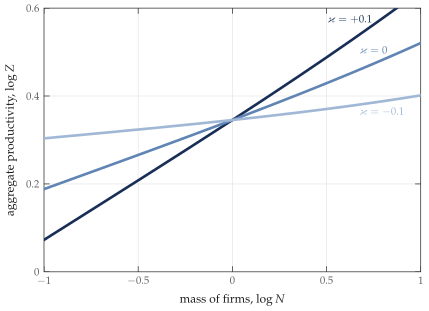
Aggregate productivity \(\log Z\) as a function of the mass of varieties \(\log N\). The parameter \(\varkappa\) controls the strength of the variety effect: \(\varkappa=0\) is our benchmark model, \(\varkappa=-0.1\) has a much weaker variety effect, \(\varkappa=+0.1\) has a much stronger variety effect.
Table I1 reports the welfare costs of markups under various alternative policy scenarios for \(\varkappa=-0.1\) and \(\varkappa=+0.1\). With \(\varkappa=-0.1\) the planner wants many fewer varieties, but with \(\varkappa=+0.1\) the planner wants many more varieties. Notice that regardless of the sign of \(\varkappa\), the welfare costs are larger than in our benchmark model. This reflects the additional inefficiency due to entry externalities in the market equilibrium. The value of \(\varkappa\) does not affect the amount of misallocation, which remains \(0.97\%\) of gross output TFP, as in our benchmark model with \(\mathcal{M}=1.15\). Nonetheless, the welfare gains from size-dependent subsidies are considerably larger. This is because the size-dependent subsidies correct both misallocation and the entry distortion and the entry distortion here is larger than in our benchmark. Although these channels are not perfectly additive, by comparing the gains from the full set of size-dependent subsidies to the gains from the optimal uniform entry subsidy, one can see that the welfare gains from correcting the misallocation distortion are between 2 and 3% in all cases — larger than than the gross output TFP loss because of the standard multiplier effect from intermediates.
| steady state comparisons, % | |||||||||
|---|---|---|---|---|---|---|---|---|---|
| \(Y\) | \(C\) | \(L\) | \(N\) | \(K\) | \(Z\) | welfare, % | |||
| \(\varkappa =-0.1\) | efficient | 42.4 | 24.4 | 9.4 | -66.9 | 72.4 | -3.7 | 17.48 | |
| uniform subsidy | 47.9 | 31.8 | 17.0 | 10.0 | 82.9 | 0.4 | 3.70 | ||
| size-dependent subsidy | -3.9 | -5.5 | -7.2 | -69.8 | -6.1 | -4.1 | 11.55 | ||
| entry subsidy | -7.5 | -8.6 | -7.8 | -66.8 | -11.0 | -4.5 | 8.66 | ||
| \(\varkappa=0.0\) | efficient | 59.6 | 44.5 | 18.0 | 20.1 | 100.4 | 4.1 | 8.67 | |
| uniform subsidy | 51.8 | 35.8 | 17.0 | 9.5 | 88.5 | 1.5 | 5.90 | ||
| size-dependent subsidy | 5.3 | 6.2 | 1.0 | 8.3 | 6.6 | 2.3 | 2.87 | ||
| entry subsidy | 6.3 | 7.4 | 2.4 | 20.0 | 8.1 | 3.0 | 0.56 | ||
| \(\varkappa =+0.1\) | efficient | 115.7 | 108.5 | 25.3 | 90.0 | 189.0 | 21.5 | 20.20 | |
| uniform subsidy | 55.3 | 39.6 | 16.9 | 9.1 | 93.8 | 2.5 | 8.01 | ||
| size-dependent subsidy | 41.7 | 50.4 | 8.5 | 71.3 | 53.7 | 17.9 | 13.74 | ||
| entry subsidy | 47.9 | 57.9 | 11.1 | 91.7 | 62.7 | 20.6 | 11.56 | ||
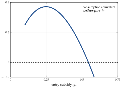
Consumption equivalent welfare gains (including transitional dynamics) as a function of the entry subsidy \(\chi_e\) for aggregate markup \(\mathcal{M}=1.15\). The welfare gains for entry subsidies reported in Table 4 are for the optimal entry subsidies, i.e., for the peak of such curves for each \(\mathcal{M}\). In our benchmark calibration there is insufficient entry in the initial distorted steady state so the optimal entry subsidy is positive. But entry subsidies that are too large lead to welfare losses.
Or the sales-weighted harmonic average, as in Edmond et al. (2015) and Grassi (2017).↩︎
For example, for the US economy De Loecker et al. (2020) estimate a sharply increasing sales-weighted average markup rising from about 1.2 in 1980 to about 1.6 in 2016. By contrast the cost-weighted average is lower and has risen by less, from about 1.1 to about 1.25. The difference reflects the increase in cross-sectional markup dispersion. We discuss these measures at length in Appendix A.↩︎
There are however standard love-of-variety gains from increasing the number of firms.↩︎
These offsetting direct and compositional effects are reminiscent of results in the trade literature, e.g., Bernard et al. (2003) and especially Arkolakis et al. (2019). We derive analogous results for Kimball and translog demand but unlike in their analysis, we do not assume from the outset that the ‘choke price’ in either demand system is binding, since this is an equilibrium outcome. For the translog case, we also provide closed-form solutions for the aggregate markup and the cutoff productivity that pins down the cross-sectional distributions of markups and market shares.↩︎
Rossi-Hansberg et al. (2020) show that while aggregate US product-market concentration has been rising since the early 1990s, concentration in geographically-specific local markets has been falling.↩︎
In our model with oligopoly, the potential number of firms per sector \(n_t(s)\) is endogenous. This problem is challenging because potential entrants anticipate their impact on a sector, and the distribution of sectoral configurations is a very high-dimensional object. By contrast in Atkeson and Burstein (2008), Edmond et al. (2015), and De Loecker et al. (2021), the potential number of firms is static and exogenous, with firms simply deciding whether to operate or not.↩︎
In this notation, a firm of size \(q_{it}(s)\) has price \(p_{it}(s)=f(q_{it}(s))\times p_t(s)d_t(s)\).↩︎
With a finite number of sectors \(S\), entry per sector \(m_t(s)\) would be IID Binomial with number of trials \(M_tS\) and success per trial \(1/S\). Taking \(S\rightarrow\infty\) this converges to a Poisson with rate parameter \(M_t\).↩︎
The aggregator \(\Upsilon(q)\) itself is given by \[ \Upsilon(q)=1+(\bar{\sigma}-1)\exp\left(\frac{1}{\varepsilon}\right)\varepsilon^{\frac{\bar{\sigma}}{\varepsilon}-1}\left[\Gamma\left(\frac{\bar{\sigma}}{\varepsilon},\frac{1}{\varepsilon}\right)-\Gamma\left(\frac{\bar{\sigma}}{\varepsilon},\frac{q^{\varepsilon/\bar{\sigma}}}{\varepsilon}\right)\right]\] where \(\Gamma(s,x):=\int_{x}^{\infty}t^{s-1}e^{-t}dt\) denotes the upper incomplete Gamma function.↩︎
Our benchmark model with monopolistic competition features identical sectors so there is no variation in outcomes between sectors. In Section 6 we consider an alternative model with oligopolistic competition which features both within- and between-sector variation in concentration. We calibrate our oligopoly model to match within-sector concentration and the sector-level relationship between markups and market shares.↩︎
This is similar to how we estimated the within-industry relationship between market shares and markups in Edmond et al. (2015) but adapted to the Kimball demand system used here.↩︎
See e.g., Atkeson et al. (2019), Barkai (2020), De Loecker et al. (2020), Gutiérrez and Phillippon (2017a, 2017b), and Hall (2018) etc. Basu (2019) surveys this literature.↩︎
We discuss the sensitivity of our results to this common slope coefficient assumption in Appendix C in the supplementary online appendix.↩︎
For multi-establishment firms we construct establishment-level markups \(\mu_{eit}(s)\) and then aggregate to firm-level markups \(\mu_{it}(s)\) weighting establishments \(e\) by their their share of the firm’s wage bill.↩︎
For our benchmark model, this elasticity is \(\alpha_t^l(s)=(1-\alpha)\zeta_t\), i.e., the elasticity of output with respect to value-added \(\zeta_t\) times the elasticity of value-added with respect to labor \((1-\alpha)\), see Appendix B.↩︎
Our results are robust to relaxing the assumption of constant returns to scale, see Appendix C in the supplementary online appendix.↩︎
We take this average to reduce the role of measurement error. These calculations also use sector-specific user costs of capital from the NBER-CES and BLS as in Foster et al. (2016).↩︎
That said, De Ridder et al. (2022) show by simulation that markups estimated using revenue data are systematically related to the true markups in their model. In this sense the revenue-based estimates are informative about markup variation even if not informative about markup levels.↩︎
See Eslava and Haltiwanger (2020) who study the life-cycle of Colombian manufacturing plants and find that markup variation plays only a small role in accounting for variation in average revenue products.↩︎
We discuss the effects of variety on aggregate productivity in more detail in Appendix I in the supplementary online appendix.↩︎
In our benchmark economy, sectors \(s\in[0,1]\) are ex post identical and we have \(d_t(s)=D_t\), \(y_t(s)=Y_t\), \(p_t(s)=1\), \(z_t(s)=Z_t\), \(n_t(s)=N_t\) etc.↩︎
See (2003) and (2019) who show that the markup distribution is invariant to changes in trade costs in models where variable markups arise due to limit pricing and monopolistic competition with non-CES demand, respectively.↩︎
This higher super-elasticity is almost exactly what we find in an alternative parameterization where we infer the super-elasticity from a log-linear approximation to (59). In this alternative log-linear specification the quality effect would be absorbed by firm fixed effects, see Appendix C in the supplementary online appendix for details.↩︎
As discussed in Appendix F in the supplementary online appendix, the model with Kimball demand is qualitatively similar to translog demand in that for Kimball demand the aggregate markup \(\mathcal{M}_t\) is also invariant to \(N_t\) if there are positive selection effects. But in our benchmark calibration of the Kimball model, there are no selection effects and changes in \(N_t\) do change \(\mathcal{M}_t\) albeit by negligible amounts.↩︎
(Rodriguez-Lopez 2011) derives a related result, solving for the average markup \(\int \mu_t(z)\,dG(z)\) with translog demand and Pareto productivity and shows that this depends only on the Pareto tail \(\xi\). Also related, Arkolakis et al. (2019) show that with translog demand and Pareto productivity the univariate distribution of markups \(\text{Prob}[\mu'\leq \mu]\) depends only on the Pareto tail \(\xi\). Our key analytic contribution is to explicitly compute the aggregate markup, the sales-weighted harmonic average \(\mathcal{M}_t=\big(N_t \int (\omega_t(z)/\mu_t(z)) dG(z)\big)^{-1}\), which, as we have stressed throughout, is the key wedge in the optimality conditions of the representative firm.↩︎
In this oligopoly model, sectors are ex post heterogeneous so we put back dependence on \(s\) in the notation.↩︎
Other applications of this oligopoly setup, e.g., Atkeson and Burstein (2008), Edmond et al. (2015), and De Loecker et al. (2021), treat the number of potential producers as exogenous.↩︎
The CR4 and CR20 are reported in Panel A of Figure 4 while the regression coefficient \(\hat{b}\) is from Table 2 baseline column 3 in Autor et al. (2020).↩︎
This amount of dispersion in sector-level markups is however less costly, because of the low elasticity of substitution \(\eta\) between sectors. The amount of markup dispersion within sectors is more important.↩︎
Since the initial steady state has too many firms, the optimal entry subsidy is a tax.↩︎
Recall that we choose the sunk entry cost \(\kappa\) to normalize \(N=1\) in the initial distorted steady state.↩︎
A steady-state calculation including capital would overstate the costs of markups because it would ignore the deferred consumption required to build up the efficient capital stock.↩︎