1 Introduction
Will improvements in information technologies help in overthrowing autocratic regimes? Optimists on this issue stress the role of new technologies in facilitating coordination and in improving information about a regime’s intentions and vulnerabilities. The “Arab Spring” of uprisings against regimes in Tunisia, Egypt, Libya and elsewhere that began in December 2010 has led to widespread discussion of the role of modern social media such as Facebook, Twitter, Skype and YouTube in facilitating regime change. Similar discussion followed the use of such technologies during the demonstrations against the Iranian regime in June 2009 (e.g., Musgrove 2009; Kirkpatrick 2011).
But optimism about the use of new technologies in putting autocratic regimes under sustained pressure is hardly new; social media is only the latest technology to be viewed as a catalyst for regime change. Simple internet access, cell phones, satellite television, radio and newspaper have all been viewed as potential catalysts too. And while information optimism has a long and somewhat mixed history, it is also worth bearing in mind that the relationship between information technologies and autocratic regimes has a prominent dark side. Perhaps the most well known examples are the use of mass media propaganda by Nazi Germany and the Soviet Union. Moreover it has become increasingly clear that recent breakthroughs in information technology also provide opportunities for autocracies. During the Iranian demonstrations, technologies like Twitter allowed the regime to spread rumors and disinformation (Esfandiari 2010). Similarly, the Chinese regime’s efforts to counter online organization make use of the exact same technologies that optimists hope will help in bringing regime change (Kalathil and Boas 2003; Fallows 2008; Morozov 2011).
So, should we be optimistic that recent breakthroughs in information technology will lead to the collapse of present-day autocratic regimes? To help address this question, I develop a simple model of information and regime change. While stylized, the model provides a number of insights into the ways in which a regime’s chances of survival are affected by changes in information technology. In particular, the model implies the degree of scale economies, if any, in the regime’s control over multiple sources of information plays a crucial role in determining whether an information revolution is likely to bring about regime change. For example, suppose an information revolution consists of technologies such as newsprint, radio, and cinema that are relatively easily centralized in the sense that, by investing in a large fixed propaganda establishment, the regime can then exert influence over additional newspapers, radio stations or cinemas at low marginal cost. Then the regime may have sufficiently strong economies of scale in information control that its chances of survival will increase. By contrast, if the technology is more decentralized, so that there are diseconomies of scale in information control, then the model predicts the regime will become easier to overthrow as the number of sources of information increases.
Section 2 outlines the model. There is a single regime and a large number of citizens with heterogeneous information. Citizens can participate in an attack on the regime or not. If enough do, the regime is overthrown. The regime’s ability to withstand an attack is given by a single parameter, the regime’s type. Citizens are imperfectly informed about the regime’s type and may coordinate either on overturning the regime or not. The regime is informed about its type and seeks to induce coordination on the status quo. It does this by taking a costly hidden action which influences the distribution of signals so that citizens receive biased information that, taken at face-value, suggests the regime is hard to overthrow. Citizens are rational and internalize the regime’s incentives when forming their beliefs.
Section 3 gives the paper’s first main result: this coordination game with endogenous information manipulation has a unique perfect Bayesian equilibrium. Section 4 then turns to the implications of changes in information precision, holding the number of sources of information fixed. The second main result of the paper is that the regime’s information manipulation increases the regime’s ex ante chances of surviving when the intrinsic per-unit signal precision is sufficiently high. If this per-unit precision is sufficiently high, then the regime survives in all circumstances where it is possible for the regime to survive. Section 5 then allows for an increase in the number of signals, which simultaneously (i) increases the total signal precision and (ii) increases the regime’s costs of information manipulation. These two effects have offsetting implications for the regime’s chances of surviving. The third main result of the paper is that the net effect of an increase in the number of signals is to reduce the regime’s chances of surviving — unless there are strong economies of scale in information control. This section also discusses the model’s predictions in light of the historical relationship between autocracies and information control. Section 6 considers two extensions. Section 7 concludes. All proofs are in the appendix. A supplementary online appendix contains further extensions and discussion.
Effective information manipulation. Perhaps the most interesting feature of the model is that the regime’s information manipulation — a form of signal-jamming — can be effective in equilibrium. The regime is informed and takes a type-specific hidden action that cannot be directly observed by the individual citizens receiving the information. While the citizens know, in equilibrium, the function mapping the regime’s type into its hidden action, they must infer the specific value of the action jointly with making inferences about the type itself. This distinguishes the setup from standard career concerns models, such as Holmström (1999), where the information sender is uninformed and chooses a single action to maximize its expected payoff, thereby making it easy for receivers to deduce any bias in their signals and respond accordingly. In my model, the extent to which signal-jamming is effective depends on the signal precision. If signals are precise, clustered tightly about the mean, then it takes only a small amount of bias to deliver a large shift in aggregate behavior, and, consequently, signal-jamming can be especially effective.
Moreover, the signal-jamming effect is amplified by the fact that information receivers are playing a coordination game. It is common knowledge that the regime has the ability to manipulate information and that any equilibrium manipulation tends to reduce the mass of citizens who participate in an attack. Since individual actions are strategic complements, at the margin this reduces every individual’s incentives to participate in an attack. In short, the strategic complementarities amplify the effectiveness of any bias the regime is able to impart. These coordination aspects of the model also distinguish the setup from standard models of strategic information transmission, such as Crawford and Sobel (1982), that focus on a single sender and single receiver. As in such models, different types of senders are able to partially pool in equilibrium. But whereas in Crawford and Sobel (1982) such pooling takes the form of different sender types choosing the same observable (and payoff irrelevant) message, here it takes the form of different regimes choosing different but unobservable actions in a way that allows lower types to mimic the strength of higher types and thereby reduce the size of the attack against them.
Uniqueness. The model is also closely related to Angeletos et al. (2006). Both my model and theirs start with a coordination game with imperfect information — often referred to as a global game1 — and to that add an informed policy-maker whose actions make information endogenous. Angeletos et al. (2006) show that an endogenous information structure can lead to equilibrium multiplicity even if the underlying global game has a unique equilibrium. My model features a unique equilibrium despite its endogenous information structure and in that sense is more reminiscent of standard global games. The key reason for the uniqueness in my model relative to theirs is that in my setting the endogenous signals are a monotone function of the regime’s type whereas in Angeletos et al. (2006) the endogenous signals are a non-monotone function that gives information receivers more common belief as to whether the status quo is likely to prevail or not. The greater common belief in their setting makes it easier to sustain multiple equilibria.
In short, this paper provides a framework with a form of costly noisy signaling that, by contrast with the indeterminacies of many signaling models, instead features determinate outcomes of the kind familiar from standard global games.
2 Model of Information Manipulation and Regime Change
There is a unit mass of ex ante identical citizens, indexed by \(i\in [0,1]\). The citizens face a regime that seeks to preserve the status quo. Each citizen decides whether to participate in an attack on the regime, \(s_i=1\), or not, \(s_i=0\). The aggregate attack is \(S:=\int_{0}^{1}s_{i}di\). The type of a regime \(\theta\) is its private information. The regime is overthrown if and only if \(\theta<S\).
Citizen payoffs. The payoff to a citizen is given by \[\tag{1} u(s_i,S,\theta) = (\mathbbm{1}\{\theta<S\} - p) s_i\] where \(\mathbbm{1}\{\cdot\}\) denotes the indicator function and where \(p>0\) is the opportunity cost of participating in an attack. A citizen will participate, \(s_i=1\), whenever they expect regime change to occur with more than probability \(p\). To focus on scenarios where individual decisions are not trivial, I also assume that \(p<1\). Otherwise, if \(p\geq 1\), it is optimal for an individual to not participate independent of \(\theta\) and \(S\). With \(p<1\) the individual \(s_i\) and aggregate \(S\) are strategic complements: the more citizens participate in an attack, the more likely it is that the regime is overthrown and so the more likely it is that any individual also participates.
Citizen information and media outlets. Citizens begin with common priors for \(\theta\), specifically the improper uniform on \(\mathbb{R}\). Citizens obtain information about the regime from \(n\geq1\) identical media outlets. Each outlet \(j=1,...,n\) releases a report \(y\) and each citizen observes that report with idiosyncratic noise. In particular, citizen \(i\) receives \(n\) signals of the form \(x_{ij} = y + \varepsilon_{ij}\) where the noise \(\varepsilon_{ij}\) is jointly IID normal across citizens and media outlets with mean zero and precision \(\hat{\alpha}>0\). Crucially, media outlets report the regime’s apparent strength \(y=\theta+a\), the sum of the regime’s true type \(\theta\) plus an action \(a\geq0\) chosen by the regime in an effort to convey a biased impression of how difficult it will be to overthrow.2 Citizens cannot directly observe this action \(a\) and must infer it jointly with inferring \(\theta\) itself.
The average signal of citizen \(i\) is \(x_i:=\frac{1}{n}\sum_{j=1}^n x_{ij}\), which is normal with mean \(y=\theta+a\) and precision \(\alpha:=n\hat{\alpha}\), proportional to \(n\). Given the regime’s apparent strength \(y\), the density of average signals is \[\tag{2} f(x_i \,|\, y) := \sqrt{\alpha}\phi(\sqrt{\alpha}(x_i-y)), \qquad y=\theta+a\] where \(\phi(\cdot)\) denotes the standard normal PDF. Since the average signal is a sufficient statistic, I simply refer to this as the citizen’s signal for short.
Regime’s costs of information manipulation. The regime’s choice of hidden action \(a\) is made after observing \(\theta\), i.e., the regime is informed. The action \(a\) enters the citizens’ \(n\) signals symmetrically with cost \(C(a,n)\) to the regime. If \(a=0\), the regime pays no cost, \(C(0,n)=0\) for all \(n\). But for \(a>0\), the cost is strictly increasing in both arguments, \(C_a > 0\) and \(C_n > 0\), and convex in the hidden action, \(C_{aa}\geq 0\). An important special case is \(C(a,n)=c(n)a\), i.e., where the marginal cost of taking action \(a\) is a constant \(c(n)>0\), with \(c(n)\) increasing in \(n\). To simplify notation, I suppress the exogenous parameter \(n\) and simply write the cost function \(C(a)\) whenever no confusion ought to arise.
Regime’s payoffs. The gross benefit to the regime \(B(\theta,S)\) depends on whether it survives or not. If \(\theta<S\) the regime is overthrown and obtains an outside option normalized to zero. Otherwise, if \(\theta\geq S\), the regime obtains a gross benefit \(\theta-S\) from remaining in power. The key assumption here is that the benefit is separable in \(\theta\) and \(S\). Given separability, the linearity in \(\theta\) and \(S\) is without further loss of generality and simply represents a normalization of the type. The benefit is strictly decreasing in \(S\), i.e., the regime wants to minimize the costs of unrest and so wants \(S\) small even when it survives.
The net payoff to a regime can therefore be written \[\tag{3} B(\theta,S)-C(a) = \max[0\,,\,\theta-S] - C(a)\] Observe that if \(\theta<S\), the regime will choose \(a=0\) and thereby obtain a net payoff of zero.
Equilibrium. A symmetric perfect Bayesian equilibrium of this model consists of individual beliefs \(\pi(\theta\,|\, x_i)\) and participation decisions \(s(x_i)\), an aggregate attack \(S(y)\), and regime actions \(a(\theta)\) such that: (i) a citizen with information \(x_i\) rationally takes into account the manipulation \(y(\theta)=\theta+a(\theta)\) when forming their posterior beliefs, (ii) given these beliefs, \(s(x_i)\) maximizes individual expected utility, (iii) the aggregate attack is consistent with the individual decisions, and (iv) the actions \(a(\theta)\) maximize the regime’s payoff given the aggregate attack. In equilibrium, the regime is overthrown if \(\theta<S(y(\theta))\) and otherwise survives.
Standard global game benchmark. If there are no hidden actions, the analysis reduces to that of a standard global game. In particular, if \(a(\theta)=0\) for all \(\theta\), then each citizen has exogenous signal \(x_i= \theta + \varepsilon_i\) and there is a unique equilibrium, as in Carlsson and Damme (1993) and Morris and Shin (1998). In this equilibrium, strategies are threshold rules: there is a unique \(\theta^*_{\text{MS}}\) such that the regime is overthrown for \(\theta <\theta^*_{\text{MS}}\) and a unique signal \(x^*_{\text{MS}}\) such that a citizen participates for \(x_i<x^*_{\text{MS}}\). These thresholds are given by:
Morris-Shin Benchmark. The equilibrium thresholds \(x^*_{\text{MS}},\theta^*_{\text{MS}}\) simultaneously solve \begin{align} \text{Prob}[\theta<\theta^*_{\text{MS}}\,|\,x^*_{\text{MS}} ] = \Phi(\sqrt{\alpha}(\theta^*_{\text{MS}}-x^*_{\text{MS}})) &=p \tag{4} \\ \text{Prob}[x_i < x^*_{\text{MS}} \, | \, \theta^*_{\text{MS}}] = \Phi(\sqrt{\alpha}(x^*_{\text{MS}}-\theta^*_{\text{MS}})) &=\theta^*_{\text{MS}}\tag{5} \end{align} where \(\Phi(\cdot)\) denotes the standard normal CDF and \(p\) is the individual opportunity cost of attacking. In particular, \(\theta^*_{\text{MS}}=1-p\), independent of \(\alpha\), and \(x^*_{\text{MS}}=1-p-\Phi^{-1}(p)/\sqrt{\alpha}\).
The first condition says that if the regime’s threshold is \(\theta^*_{\text{MS}}\), the marginal citizen with signal \(x_i=x^*_{\text{MS}}\) expects regime change with exactly probability \(p\). The second says that if the signal threshold is \(x^*_{\text{MS}}\), a regime with \(\theta=\theta _{\text{MS}}^{\ast }\) will be indifferent to abandoning its position.
3 Unique Equilibrium with Information Manipulation
The first main result of this paper is that there is a unique equilibrium:
Proposition 1. There is a unique perfect Bayesian equilibrium. The equilibrium is monotone in the sense that there exist thresholds \(x^*\) and \(\theta^*\) such that \(s(x_i)=1\) for \(x_i<x^*\) and zero otherwise, while the regime is overthrown for \(\theta<\theta^*\) and not otherwise.
A detailed proof is given in Appendix A. Briefly, the proof involves first showing (i) that there is a unique equilibrium in monotone strategies, and (ii) that the unique monotone equilibrium is the only equilibrium which survives the iterative elimination of interim strictly dominated strategies. Here in the main text I briefly characterize the equilibrium.
3.1 Equilibrium Characterization
Let \(\hat{x}\) denote a candidate for the citizens’ threshold and let \(\Theta(\hat{x})\) and \(a(\theta,\hat{x})\) denote candidates for the regime’s threshold and hidden actions given \(\hat{x}\).
Regime problem. Since citizens participate \(s(x_i)=1\) for \(x_i<\hat{x}\), for any given \(\hat{x}\) the aggregate attack facing a regime of apparent strength \(y\) is simply \begin{align} S(y) = \Phi(\sqrt{\alpha}(\hat{x}-y)),\qquad y=\theta+a \tag{6} \end{align} (using the form of the signal density given in (2) above). Since the regime is overthrown for \(\theta<\Theta(\hat{x})\), hidden actions are \(a(\theta,\hat{x})=0\) for all \(\theta<\Theta(\hat{x})\), otherwise the regime would be incurring a cost but receiving no benefit. For all \(\theta\geq\Theta(\hat{x})\), the regime chooses \[\tag{7} a(\theta,\hat{x})\in\operatornamewithlimits{argmin}_{a\geq0}\left[\Phi(\sqrt{\alpha}(\hat{x}-\theta-a))+C(a)\right]\] A key step in proving equilibrium uniqueness is to recognize that hidden actions are given by \(a(\theta,\hat{x})=A(\theta-\hat{x})\), where the auxiliary function \(A:\mathbb{R}\rightarrow\mathbb{R}_+\) is exogenous and in particular does not depend on the citizen threshold \(\hat{x}\). This function is defined by \[\tag{8} A(t):=\operatornamewithlimits{argmin}_{a\geq0} \left[\Phi(\sqrt{\alpha}(-t-a))+C(a) \right]\] The regime threshold \(\Theta(\hat{x})\) is then found from the indifference condition \[\tag{9} \Theta(\hat{x}) = \Phi(\sqrt{\alpha}(\hat{x}-\Theta(\hat{x})-A(\Theta(\hat{x})-\hat{x}))) + C(A(\Theta(\hat{x})-\hat{x}))\] This condition requires that total costs equal total benefits at the extensive margin. For any given candidate citizen threshold \(\hat{x}\), equations (8)-(9) determine the regime threshold \(\Theta(\hat{x})\) and hidden actions \(a(\theta,\hat{x})=A(\theta-\hat{x})\) solving the regime’s problem.
Citizen problem. An individual participates only if they believe the regime will be overthrown with probability at least \(p\). Given \(\hat{x}\) and the solution to the regime’s problem, the posterior probability of regime change for an individual with arbitrary signal \(x_i\) is \[ \text{Prob}[\theta<\Theta(\hat{x})\;|\;x_i,\,a(\cdot,\hat{x})] := \frac{\int_{-\infty}^{\Theta(\hat{x})}\sqrt{\alpha}\phi(\sqrt{\alpha}(x_i-\theta))\,d\theta}{\int_{-\infty}^{\infty}\sqrt{\alpha}\phi(\sqrt{\alpha}(x_i-\theta'-a(\theta',\hat{x})))\,d\theta'}\] (using \(a(\theta,\hat{x})=0\) for all \(\theta<\Theta(\hat{x})\) in the numerator). Writing the hidden actions in terms of the auxiliary function \(a(\theta,\hat{x})=A(\theta-\hat{x})\), evaluating at \(x_i=\hat{x}\), and then equating the result to the opportunity cost \(p\) gives the indifference condition characterizing the citizen threshold \[\tag{10} \frac{\int_{-\infty}^{\Theta(\hat{x})}\sqrt{\alpha}\phi(\sqrt{\alpha}(\hat{x}-\theta))\,d\theta}{\int_{-\infty}^{\infty}\sqrt{\alpha}\phi(\sqrt{\alpha}(\hat{x}-\theta'-A(\theta'-\hat{x})))\,d\theta'}=p\]
Monotone equilibrium. As shown in Appendix A, there is a unique monotone equilibrium with thresholds \(x^*\) and \(\theta^*\) simultaneously solving conditions (9) and (10). The regime’s equilibrium hidden actions are then given by \(a(\theta)=A(\theta-x^*)\) using the auxiliary function from (8). A key step in the proof is showing that the posterior probability on the left hand side of equation (10) depends only on the difference \(\Theta(\hat{x})-\hat{x}\) and is monotone increasing in this argument so that (10) can be solved for a unique difference \(\theta^*-x^*\). Similarly, the right hand side of (9) only depends on the difference \(\Theta(\hat{x})-\hat{x}\) so we can take the unique solution \(\theta^*-x^*\) from (10) and plug it into the right hand side of (9) to determine \(\theta^*\) separately.
The appendix goes on to show that this monotone equilibrium is the only equilibrium.
4 Equilibrium Information Manipulation
The most interesting implication of this model is that the regime’s information manipulation — or signal-jamming — can be an effective tool for increasing the regime’s ex ante chances of surviving. Section 4.1 begins the analysis by showing that the regime’s policy \(y(\theta)\) is monotone in \(\theta\), a general result that obtains independent of precise details of the equilibrium. Section 4.2 then specializes to the case of a linear cost function. This permits a simple characterization of the entire equilibrium, not just the signal-jamming policy. Section 4.3 then shows that, for a given number of signals \(n\), the regime’s signal-jamming will be effective in equilibrium if the per-unit signal precision \(\hat{\alpha}\) is sufficiently high. Section 4.4 provides further intuition and explains how these results relate to standard models in the literature.
4.1 Signal-Jamming Policy
To understand the regime’s signal-jamming problem intuitively, it is helpful to recast the problem in slightly more general terms. In particular, let \(B(\theta,S)\) denote the regime’s gross benefit from surviving and let \(S(y)\) denote the aggregate attack facing a regime that chooses apparent strength \(y\geq\theta\). For the moment, \(S(y)\) can be anything — no equilibrium properties need to be imposed at all. In these general terms, the regime’s policy is \[\tag{11} y(\theta)\in\operatornamewithlimits{argmax}_{y\geq \theta} \left [B(\theta,S(y)) - C(y-\theta) \right]\] with \(B(\theta,S)=0\) whenever the regime is overthrown. We then have:
Proposition 2. If \(B(\theta,S)\) satisfies the Spence-Mirrlees sorting condition \(B_{\theta S}\leq 0\), then for any aggregate attack \(S(y)\) the solution \(y(\theta)\) to (11) is increasing in \(\theta\).
The proof is given in Appendix A. The key steps are to observe (i) that for given \(\theta\), at any interior solution higher values of \(y\) cost more and so will be chosen only if they reduce \(S(y)\), and (ii) since \(B(\theta,S)\) satisfies a sorting condition in \(\theta\) and \(S\), stronger regimes are at least weakly better off from a smaller attack than are weaker regimes,3 hence stronger regimes are more willing, at the margin, to pay the cost of choosing a larger \(y\).
This monotonicity result is intuitive, but, since the form of \(S(y)\) is left open, we do not yet know if this policy will be effective in equilibrium.
4.2 Equilibrium with Linear Costs
To study the equilibrium problem, I first specialize to the case of linear costs, \(C(a):=c\,a\) for some constant \(c>0\). This gives rise to a simple form of signal-jamming and permits an exact characterization of the conditions under which the signal-jamming is effective.
Overview of the regime’s problem. With linear costs, if the choice of \(y\) is to induce survival it must minimize \(S(y)+cy\) subject to the constraint \(y\geq \theta\). Since the first order condition for interior solutions is \(-S'(y)=c\), all regimes with interior solutions choose the same apparent strength \(y^*\). Corner solutions can arise for two reasons: (i) for all \(\theta\) such that \(\theta<S(y^*)+c(y^*-\theta)\) the regime is too weak to sustain the cost of taking \(y^*\) and hence is overthrown, and (ii) for all \(\theta\geq y^*\) the innate strength of the regime is sufficiently high that they do not need to undertake any costly manipulation (i.e., the non-negativity constraint \(y\geq \theta\) is binding). All regimes at a corner simply have apparent strength equal to actual strength, \(y(\theta)=\theta\). All regimes that are at an interior solution have \(y(\theta)=y^*\). In short,
\[\tag{12} y(\theta) = \left\{\begin{array}{ll} \quad \theta & \text{if $\theta\notin[\theta^*,\theta^{**})$} \\ \quad y^* \qquad & \text{if $\theta\in[\theta^*,\theta^{**})$} \\ \end{array}\right.\] The cutoff \(\theta^*\) is just the threshold above which the regime survives and is implicitly determined by the indifference condition \(\theta^* = S(y^*) + c(y^*-\theta^*)\). The higher cutoff \(\theta^{**}\) is simply equal to the apparent strength \(y^*\) since it is the smallest regime type for which the non-negativity constraint \(y^*\geq \theta\) is binding. Figure 1 illustrates. Observe that the lower cutoff \(\theta^*\) necessarily lies in \([0,1]\) since no regime with \(\theta<0\) can survive and any regime with \(\theta>1\) must survive. The upper cutoff \(\theta^{**}\) may be greater than \(1\) though. Even when the regime survives, it prefers \(S\) to be small (to reduce the costs associated with insurrections).
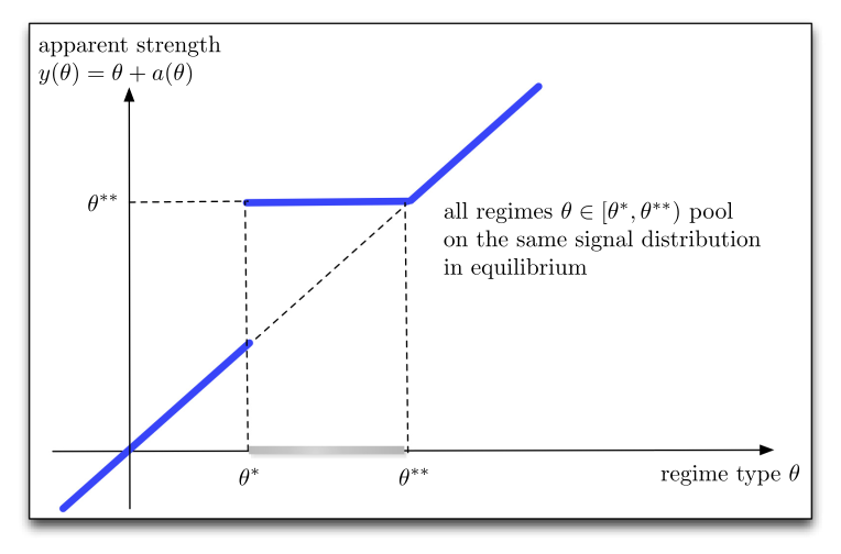
Apparent strength \(y(\theta)=\theta+a(\theta)\) when the regime has linear costs of manipulation. All regimes with \(\theta<\theta^*\) are overthrown. All regimes with \(\theta\in[\theta^*,\theta^{**})\) choose the same apparent strength \(y^*=\theta^{**}\) and thus generate the same signal distribution in equilibrium. They mimic a stronger regime \(\theta^{**}\) and generate signals for the citizens that are (locally) uninformative about \(\theta\).
To summarize, regimes that are sufficiently weak and that will be overthrown, \(\theta<\theta^*\), do not engage in any manipulation. Regimes that are sufficiently strong, \(\theta\geq\theta^{**}\), have enough innate ability to resist an attack that they do not engage in any costly manipulation to shore up their position. Only intermediate regimes \(\theta\in[\theta^*,\theta^{**})\) find it worthwhile to pay the costs of manipulation in equilibrium and all these intermediate regimes mimic the strength of a strong regime, \(\theta^{**}\).
No manipulation, Morris-Shin outcome. Intuitively, when the cost of manipulation is sufficiently high, no regime will find it worthwhile to manipulate and the unique equilibrium will coincide with the Morris-Shin outcome. Since the aggregate attack is \(S(y)=\Phi(\sqrt{\alpha}(x^*-y))\), the first order necessary condition \(-S'(y)=c\) can be written \[\tag{13} \sqrt{\alpha} \phi(\sqrt{\alpha}(x^*-y^*)) = c\] Observe that \(c/\sqrt{\alpha}\) must be sufficiently small for this condition to have a solution.4 In particular, a necessary condition for the existence of an interior solution is that \(c/\sqrt{\alpha}< \phi(0)\) where \(\phi(0)=1/\sqrt{2\pi}\approx0.399\) is the maximum value of the standard normal density. If \(c/\sqrt{\alpha}\geq \phi(0)\), then the signal precision \(\alpha\) is too low relative to the cost of manipulation and all regimes are at a corner with \(y(\theta)=\theta\). In this case, \(\theta^*=\theta_{\text{MS}}^* = 1-p\) and \(\theta^{**}=\theta^*\). By contrast, if the signal precision is high, some regimes will engage in information manipulation.
Active manipulation. In particular, let \(\underline{\alpha}(c):=(c/\phi(0))^2\) denote the smallest precision such that (13) has a solution. Then all regimes that manipulate choose apparent strength \[\tag{14} y^* = x^* + \gamma\] where the parameter \(\gamma\) solves \(\sqrt{\alpha}\phi(\sqrt{\alpha}\gamma)=c\), that is \[\tag{15} \gamma= \sqrt{\frac{1}{\alpha}\log\left(\frac{\alpha}{\underline{\alpha}(c)}\right)}>0,\qquad \alpha>\underline{\alpha}(c)\] The signal-jamming is acute. All regimes that manipulate information pool on the same distribution of signals, i.e., all regimes \(\theta\in[\theta^*,\theta^{**})\) generate a mean of \(y^*=\theta^{**}\) with signals \(x_i = y^* + \varepsilon_i\) that are locally completely uninformative about \(\theta\).
Size of the attack. Now let \(S(y(\theta))\) denote the size of the aggregate attack facing a regime of type \(\theta\) when the signal-jamming has this form. Using (12) and (14), the attack is \[\tag{16} S(y(\theta)) = \left\{\begin{array}{ll} \quad \Phi(\sqrt{\alpha}(x^*-\theta)) \qquad & \text{if $\theta\notin[\theta^*,\theta^{**})$} \\ \quad \Phi(-\sqrt{\alpha}\gamma) & \text{if $\theta\in[\theta^*,\theta^{**})$} \\ \end{array}\right.\] Manipulation to convey a higher apparent strength causes the size of the attack to drop discontinuously at the regime threshold \(\theta^*\). As shown in Figure 2, at \(\theta^*\) the size of the attack jumps discretely from \(\Phi(\sqrt{\alpha}(x^*-\theta^*))\) down to the lower value \(\Phi(\sqrt{\alpha}(x^*-y^*))=\Phi(-\sqrt{\alpha}\gamma)\). All regimes that manipulate face the same-sized attack, \(\Phi(-\sqrt{\alpha}\gamma)\).
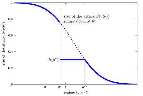
All regimes with \(\theta\in[\theta^*,\theta^{**})\) choose the same apparent strength \(y^*=\theta^{**}=x^*+\gamma\) and consequently face the same sized attack \(S(y^*)=\Phi(-\sqrt{\alpha}\gamma)\). All regimes that do not manipulate have \(y(\theta)=\theta\) and face the attack \(S(y(\theta))=\Phi(\sqrt{\alpha}(x^*-\theta))\). Observe that the attack is continuous at the upper boundary \(\theta^{**}\).
Is manipulation effective in equilibrium? Thus, as in classic signaling games, the regime is able to send a (noisy) signal in equilibrium and this enables some weaker regime types to pool with stronger regime types. But, at the risk of repetition, this pooling tells us nothing about whether the signal-jamming is effective in equilibrium. It may be that the only regimes that are able to imitate stronger regime types are those regimes that would have survived in the absence of the signal-jamming technology. Moreover, it may be that some weak regimes that would survive if they could commit to not use manipulation are overthrown because they cannot make that commitment. Put differently, the discussion so far has taken the thresholds \(\theta^*\) and \(\theta^{**}\) as given. But these thresholds are endogenous and, in principle, may shift strongly against the regime so that in equilibrium information manipulation is ultimately ineffective.
It turns out that manipulation is effective when the per-unit signal precision is sufficiently high. But to see this we have to solve the rest of the model.
Solving the model with linear costs. To complete the solution, recall that an individual citizen participates if they believe the regime will be overthrown with posterior probability at least \(p\), that is, if \(\text{Prob}[\theta<\theta^*\,|\, x_i, y(\cdot)] \geq p\). For the marginal citizen with signal \(x_i=x^*\) this condition holds with equality so that \[ \text{Prob}[\theta<\theta^*\,|\, x^*, y(\cdot)] = \frac{\int_{-\infty}^{\theta^*} \sqrt{\alpha}\phi(\sqrt{\alpha}(x^*-\theta))\,d\theta}{\int_{-\infty}^{\infty} \sqrt{\alpha}\phi(\sqrt{\alpha}(x^*-y(\theta)))\,d\theta} = p\] (since \(y(\theta)=\theta\) for \(\theta<\theta^*\)). After collecting terms \[\tag{17} \Phi[\sqrt{\alpha}(\theta^*-x^*)] = \frac{p}{1-p} \int_{\theta^*}^{\infty} \sqrt{\alpha}\phi(\sqrt{\alpha}(x^*-y(\theta)))\,d\theta\] For the special case of linear costs, the integral on the right hand side can be calculated using the first order condition (13), giving \[\tag{18} \int_{\theta^*}^{\infty} \sqrt{\alpha}\phi(\sqrt{\alpha}(x^*-y(\theta)))\,d\theta = (x^*-\theta^*+\gamma)c+\Phi(-\sqrt{\alpha}\gamma)\] (since \(y(\theta)=\theta\) for \(\theta\geq\theta^{**}\) and \(\theta^{**}=y^*=x^*+\gamma\)). Plugging this back into (17) gives \[\tag{19} \Phi[\sqrt{\alpha}(\theta^*-x^*)] = \frac{p}{1-p}\left[(x^*-\theta^*+\gamma)c+\Phi(-\sqrt{\alpha}\gamma)\right]\] It is straightforward to show that there is a unique threshold difference \(\theta^*-x^*\) that solves this equation. The regime threshold \(\theta^*\) is then determined using the indifference condition (9) which, with linear costs, can likewise be written \[\tag{20} \theta^* = (x^*-\theta^*+\gamma)c + \Phi(-\sqrt{\alpha}\gamma)\] where the difference \(\theta^*-x^*\) on the right hand side is uniquely determined by (19) above.
With the equilibrium thresholds \(x^*,\theta^*\) determined by (19)-(20), we can now derive the conditions under which information manipulation is effective for the regime.
4.3 Effectiveness of Information Manipulation
I measure the effectiveness of signal-jamming by its ability to reduce the regime’s threshold \(\theta^*\) below the Morris-Shin benchmark \(\theta_{\text{MS}}^*=1-p\). A lower \(\theta^*\) increases the regime’s ex ante survival probability by making it more likely that nature draws a \(\theta\geq\theta^*\). In principle, it might be the case that lower \(\theta^*\) is achieved through large, costly, actions that give the regime a lower net payoff than they would achieve in the Morris-Shin world. But it turns out that, for sufficiently high signal precision, the fall in \(\theta^*\) also represents a genuine increase in payoffs.
In this section I focus on results holding fixed the number of signals \(n\) (and hence holding fixed the regime’s cost function) so that an increase in the per-unit precision \(\hat{\alpha}\) is identical to an increase in the total precision \(\alpha=n\hat{\alpha}\). Since these results hold \(n\) fixed but allow for any marginal cost \(c>0\) there is no loss of generality in setting \(n=1\) so that \(\alpha=\hat{\alpha}\). In Section 5 below I return to the case of a change in the number of signals \(n\) that simultaneously changes both the total precision of information and the regime’s cost function.
Effective manipulation when signal precision is high. The main result here is:
Proposition 3. For signal precision \(\alpha\) sufficiently high, the regime threshold \(\theta^*\) is strictly less than the Morris-Shin benchmark \(\theta^*_{\text{MS}}=1-p\). In particular, for each \(c\) there is an \(\underline{\alpha}(c)\) such that: (i) for \(\alpha\leq\underline{\alpha}(c)\) all regimes are at a corner with \(y(\theta)=\theta\) for all \(\theta\) and \(\theta^*=\theta^*_{\text{MS}}\); otherwise (ii) for \(\alpha>\underline{\alpha}(c)\), regimes \(\theta\in[\theta^*,\theta^{**})\) are at an interior solution and there is a critical precision \(\alpha^*(c,p)\geq\underline{\alpha}(c)\) given by \[\tag{21} \alpha^{\ast}(c,p) := \underline{\alpha}(c) \exp \left(\max\left[0,\Phi^{-1}(p)\right]^2\right)\] such that \[\tag{22} \frac{\partial}{\partial \alpha} \theta^* <0 \qquad \text{for all} \qquad \alpha > \alpha^*(c,p)\] with \(\lim_{\alpha\rightarrow\infty}\theta^* = 0\), less than the Morris-Shin benchmark.
There are two cases to consider. First, when the opportunity cost of attacking the regime is low, \(p<1/2\), then all that matters is whether the signal precision \(\alpha\) is high enough to induce any regime to manipulate. If so, the regime threshold is monotonically declining in \(\alpha\) and so for all \(\alpha>\underline{\alpha}\) the regime threshold is less than the Morris-Shin benchmark. This is shown in the left panel of Figure 3. Second, if the opportunity cost of attacking the regime is high, \(p>1/2\), then the regime threshold is “single-peaked” in \(\alpha\), reaching a maximum at \(\alpha^*>\underline{\alpha}\) before declining thereafter. This is shown in the right panel of Figure 3. In either case, in the limit as \(\alpha\rightarrow\infty\), the regime threshold \(\theta^*\rightarrow 0\) for any fixed \(c\) and \(p\).
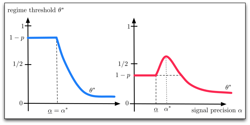
The left panel shows the case when \(p<1/2\) and the regime threshold \(\theta^*\) is monotone decreasing in the precision \(\alpha\). The right panel shows the case when \(p>1/2\) so that \(\theta^*\) is non-monotone in \(\alpha\). In both cases, for low enough precision \((\alpha<\underline{\alpha})\) the regime threshold coincides with the Morris-Shin benchmark \(\theta^*_{\text{MS}}=1-p\) while for high enough \(\alpha\) the threshold is less than \(1-p\).
Even the most fragile regimes can survive. This result is striking. As the precision becomes sufficiently high, all the regimes that can survive, do survive. To see an extreme example of this, consider an economy with opportunity cost \(p\rightarrow 0\) so that it requires almost no individual sacrifice to participate in an attack on the regime. In the Morris-Shin benchmark we would have \(\theta^*_{\text{MS}}\rightarrow 1\) and only the strongest regimes, those with \(\theta\geq 1\), can survive. But with information manipulation, we have \(\theta^*\rightarrow0\) so all regimes \(\theta\geq0\) survive even though \(p\) is very low. If information can be manipulated and signals are sufficiently precise, then even the very most fragile regimes can survive.5
Signal precision and the size of the marginal attack. To understand this result further, observe that the size of the attack facing the marginal regime, \(S(y^*)\), is always monotonically declining in the signal precision \(\alpha\). This follows immediately on plugging the expression for \(\gamma\) from (15) into (16). But there is another, perhaps more insightful, way to see this too. Recall the problem of a regime minimizing \(S(y)+cy\) with \(S(y)=\Phi(\sqrt{\alpha}(x^*-y))\). Since \(S(y)\) is strictly monotone in \(y\) we can equivalently choose \(S\) to minimize \[\tag{23} S - \frac{c}{\sqrt{\alpha}}\Phi^{-1}(S)\] with first order condition \(\phi(\Phi^{-1}(S))=c/\sqrt{\alpha}\). Any solution is independent of the citizen threshold \(x^*\) and depends only on the ratio \(c/\sqrt{\alpha}\) (rather than each parameter separately). The ratio \(c/\sqrt{\alpha}\) determines the effective cost of obtaining a given-sized attack. And, from the second order condition, the size of the attack that solves this cost minimization problem must be at least locally increasing in \(c/{\sqrt{\alpha}}\). From this point of view, we see clearly that an increase in the signal precision \(\alpha\) reduces the effective cost of obtaining a smaller attack; the more probability density is located near the mean, the easier it is for the regime to achieve a relatively large change in the size of the attack from a relatively small perturbation to the signal mean. Other things equal, a regime can achieve a smaller attack when \(\alpha\) is large.
Whenever \(\alpha>\underline{\alpha}(c)\), we can solve (23) to obtain the marginal attack \[\tag{24} S(y^*) = \Phi(-\sqrt{\alpha}\gamma) = \Phi\left(-\sqrt{\log\left(\frac{\alpha}{\underline{\alpha}(c)}\right)}\right) = \Phi\left(-\sqrt{2\log\left(\frac{\sqrt{\alpha}}{c}\phi(0)\right)}\right)\] Otherwise, for \(\alpha<\underline{\alpha}(c)\), the marginal attack is simply the Morris-Shin benchmark, \(1-p\).
This discussion highlights the special role of the effective cost parameter \(c/\sqrt{\alpha}\). When we return to the case of a variable number of signals \(n\) in Section 5 below, this will have the form \(c(n)/\sqrt{n\hat{\alpha}}\). Depending on the curvature of \(c(n)\), an increase in the number of signals may either increase, decrease, or leave unchanged the effective cost of manipulation.
Critical signal precision. If the regime did not have to pay to obtain \(y^*\), then we would be done; the reduction in the size of the marginal attack would directly translate into a reduction in \(\theta^*\). But since the manipulation is costly, the regime threshold satisfies \(\theta^* = S(y^*) + c(y^*-\theta^*)\) so that a fall in \(S(y^*)\) is not enough to guarantee that \(\theta^*\) falls as the signal precision \(\alpha\) increases. In particular, if the cost of \(y^*\) increases sufficiently faster than the size of the attack \(S(y^*)\) falls, then the threshold \(\theta^*\) increases. When this happens, there is a non-monotone relationship, as in the right panel of Figure 3. Proposition 3 establishes that this non-monotonicity in \(\alpha\) can only occur if the individual opportunity cost of attacking the regime is large (\(p>1/2\)). The critical precision \(\alpha^*\) is exactly the value of \(\alpha\) such that the marginal regime faces an attack equal to the Morris-Shin benchmark \(1-p\). Using (24), the critical precision \(\alpha^*\) solves \[\tag{25} \Phi\left(-\sqrt{2\log\left(\frac{\sqrt{\alpha^*}}{c}\phi(0)\right)}\right) = 1-p\] which can be inverted to obtain the expression in (21) above. When the signal precision is larger than \(\alpha^*\) the regime threshold \(\theta^*\) is decreasing in \(\alpha\) and is eventually less than \(1-p\).
Asymptotic results with general convex costs. While the linear cost case is particularly tractable, the key result that the regime benefits from manipulation when the signal precision is high enough is more general. In particular:
Proposition 4. For general convex cost functions \(\lim_{\alpha \rightarrow \infty }\theta^*=0^{+}\). In addition, if the cost function is strictly convex and \(C'(0)=0\), then \(\lim_{\alpha \rightarrow 0}\theta^*=1^{-}.\)
So, for high enough \(\alpha\) (again, keeping \(n\) fixed), the regime is indeed able to reduce the threshold \(\theta^*\) below the Morris-Shin benchmark \(1-p\). Of course the threshold may rise significantly above the Morris-Shin benchmark when the signal precision is low enough, just as in the linear case. A striking example of this arises when the cost function is strictly convex with \(C'(0)=0\), for example a quadratic cost \(C(a)=a^2/2\). In this case, as \(\alpha\rightarrow 0\) the regime threshold not only rises above the Morris-Shin benchmark, it is driven all the way up to \(1\), the worst possible outcome for the regime.
With linear costs, as the signal precision becomes small enough the effective cost \(c/\sqrt{\alpha}\) blows up, it is common knowledge that no regime will manipulate and so we have the Morris-Shin outcome. But with \(C'(0)=0\) the regime always has an incentive to manipulate even for very low levels of \(\alpha\), since it can always take a very small action with very small marginal cost. For low values of \(\alpha\), the regime would want to be able to commit to refrain from information manipulation. But because such commitments cannot be made, the regime is “trapped” into taking costly actions even as the precision falls. In this sense, the manipulation completely backfires on the regime when \(\alpha\) is very low.
4.4 Intuition and Further Discussion
The result that signal-jamming is effective when the precision is sufficiently high depends on two key features of the model. First, manipulation is a potentially powerful tool when the precision is high, because then most citizens have signals near the mean and it takes only a small amount of bias to deliver a large change in the aggregate attack. Second, the regime is able to use this tool, because citizens face a difficult joint coordination-and-information-filtering problem that impedes their ability to infer the amount of bias in equilibrium.
4.4.1 A Powerful Tool \(\dots\)
To see why signal-jamming is potentially powerful, observe that in the Morris-Shin benchmark the size of the aggregate attack is \(S^*_{\text{MS}}(\theta) = \Phi(\sqrt{\alpha}(x^*_{\text{MS}}-\theta))\), which approaches a step function \(\mathbbm{1}\{1-p>\theta\}\) as \(\alpha\rightarrow\infty\). A small “shock” that increased the signal mean from \(\theta\) to \(\theta+\tilde{a}\), say, would cause a shift of the step function so that the attack facing the marginal regime would fall from \(1-p\) to \(0\) and all regimes \(\theta\geq0\) would be able to survive. But this only delivers a reduction in the attack if \(\tilde{a}\) is unanticipated. If the citizens could correctly anticipate such an increase in the signal mean, then they would discount their signals appropriately.
This illustrates two points: (i) the ability to shift the mean is potentially powerful when the precision is high, for then it takes only a small amount of bias to achieve a large reduction in the size of the attack and hence a large fall in \(\theta^*\), but (ii) for this to be useful to the regime, it must be the case that the citizens are, somehow, impeded in their efforts to infer the bias.
4.4.2 \(\dots\) And the Regime Can Make Use of It
In turn, two features of the model account for the citizen’s inability to infer the bias. First, different regimes have different incentives so that given imperfect information about \(\theta\) there is also imperfect information about \(a(\theta)\). Second, citizens are imperfectly coordinated. These two features are also key differences between the model of information manipulation here and canonical environments such as the careers concerns model of Holmström (1999) and the strategic information transmission model of Crawford and Sobel (1982).
Contrast with career concerns models. Citizens know the regime’s incentives, so why can they not back out the regime’s manipulation? The short answer is that the regime is informed and takes contingent actions \(a(\theta)\) so that while citizens know the function \(a(\cdot)\) in equilibrium, they do not know \(\theta\) and hence do not know the exact value \(a(\theta)\) to extract. Instead, they must infer \(a(\theta)\) jointly with their inferences about \(\theta\) itself and cannot perfectly decompose their signal into the true \(\theta\) component and the endogenous bias component. By contrast, in standard career concerns models, such as Holmström (1999), the signal sender is itself uninformed and chooses a single action, \(\tilde{a}\) say, to maximize its expected payoff. But since this action is common to all senders, it is then straightforward for signal receivers to infer that exact amount of bias and react accordingly.
Contrast with strategic information transmission models. As in traditional models of strategic information transmission, such as Crawford and Sobel (1982), the regime here makes use of a form of partial pooling. This is most clear in the case of linear costs where all regimes \(\theta\in[\theta^*,\theta^{**})\) that intervene have the same apparent strength \(y^*\). In this model, the partial pooling is achieved by different regimes taking different unobservable actions, namely \(a(\theta)=y^*-\theta\). By contrast, in Crawford and Sobel (1982) this partial pooling takes the form of identical observable payoff-irrelevant messages.6 In related work, Kartik et al. (2007) study a model of strategic information transmission where an informed sender faces a cost of sending biased messages (or where some fraction of receivers are naive and take messages at face-value) and show that there exist fully separating equilibria (i.e., in equilibrium receivers can infer the sender’s type) and that these equilibria feature “inflated communication” in that the sender’s message is greater than the sender’s true type. The construction of these equilibria relies crucially on the assumption that the sender’s type space is unbounded above. Kartik (2009) studies a related model with costs of sending biased messages but where the type space is instead bounded above and shows that the upper bound prevents full separation. While these models feature inflated communication, by contrast with my model the sender’s information manipulation does not in fact deceive rational information receivers.
Another important difference is that information manipulation in my model is taken to influence the actions of heterogenous information receivers playing a game of strategic complementarities.
Role of strategic complementarities. To see the importance of strategic complementarities, recall that it is common knowledge that any manipulation serves to increase the regime’s apparent strength and hence to reduce the aggregate attack. Since the individual \(s_i\) and aggregate \(S\) are strategic complements, this makes each individual less likely to participate. Consequently, the size of the attack facing the marginal regime falls. Moreover, when \(\alpha\) is high, it takes only a small amount of bias to achieve a large reduction in \(S\). Knowing this makes individuals even more reluctant to participate (a standard “multiplier effect” with strategic complementarities). As \(\alpha\rightarrow\infty\), the regime threshold is driven to zero because in that limit it takes only an infinitesimal amount of bias to deter all citizens from attacking.
Role of coordination. This argument crucially relies on the citizens being imperfectly coordinated, i.e., on individuals taking the aggregate \(S\) as given. To see the importance of this, suppose to the contrary that citizens were perfectly coordinated and able to act as a single “large” agent who could force regime change for all \(\theta<1\). This agent receives a signal \(x=\theta+a+\varepsilon\) with precision \(\alpha\rightarrow\infty\). For simplicity, suppose also that costs are strictly convex. This implies \(y(\theta)\) is strictly increasing and hence can be inverted to recover \(\theta=y^{-1}(x)\). But knowing \(\theta\) the single agent can deduce any manipulation \(a(\theta)\) and discard it — so the regime has no incentive to undertake costly manipulation. Thus if citizens are perfectly coordinated, they know \(x\rightarrow\theta\) and attack if and only if \(x=\theta<1\) and all regimes \(\theta\in[0,1)\) are wiped out. By contrast, if citizens are imperfectly coordinated, all regimes \(\theta\in[0,1)\) survive. In this sense, the imperfect coordination drives the equilibrium selection in the regime’s favor (see Appendix B for more details).
Contrast with Angeletos, Hellwig and Pavan. The strategic interaction between an informed policy-maker and heterogeneous information receivers is a feature this model shares with Angeletos et al. (2006). A key difference however is that the equilibrium in my model is unique while their model features equilibrium multiplicity. The reason for this is a subtle difference in the information structure. In the version of their model closest to this paper, Angeletos et al. (2006) let individuals receive two noisy signals, (i) a pure signal of \(\theta\), and (ii) a separate signal on the endogenous action \(a(\theta)\). In my model, by contrast, individuals get one noisy observation of the sum \(y(\theta)=\theta+a(\theta)\), not separate signals for the two constituent parts. This makes an important difference.
In their setting individuals have two qualitatively different kinds of information; the pure signal is a monotone function of the policy-maker’s type, but the signal on the endogenous action \(a(\theta)\) is a non-monotone function of \(\theta\). In particular, the policy-maker chooses \(a(\theta)=a^*\) for some critical interval \(\theta\in[\theta^*,\theta^{**})\) and \(a(\theta)=\underline{a}<a^*\) otherwise. To see the importance of this, consider the benchmark version of their model where individuals observe this endogenous action without noise. In this case, the action creates common certainty that \(\theta\) is either in the critical interval \([\theta^*,\theta^{**})\) or not. This common certainty then serves as the basis of multiple possible coordinated responses. If \(a(\theta)\) is observed with unbounded idiosyncratic noise, then there is not common certainty but, so long as the noise on \(a(\theta)\) is not too great, there is enough common p-belief (in the sense of Monderer and Samet 1989) that individuals can likewise coordinate on multiple responses to their observations of the endogenous action.
In my setting, by contrast, while the actions \(a(\theta)\) may be non-monotone in \(\theta\), what matters for individual signals is the regime’s apparent strength \(y(\theta)=\theta+a(\theta)\) which, from Proposition 2, is monotone in \(\theta\). Put differently, in their setting the actions \(a(\theta)\) simply are the signal mean, whereas in my setting the actions are only part of the signal mean. The monotonicity of the signal is the key force driving equilibrium uniqueness in my setting; with monotonicity, there is not enough common p-belief to coordinate on multiple responses.
Alternative models of information manipulation. In my model the regime’s information manipulation takes a particularly simple form, namely shifting the signal mean at a cost. Marinovic (2011) considers a related model where, with some fixed probability, an informed sender receives the opportunity to send a biased message (at no cost) but with complementary probability is instead compelled to report the truth. Information receivers are uninformed about both the sender’s type and whether the sender has the opportunity to manipulate information. In equilibrium, a sender who has the opportunity to manipulate uses a mixed strategy (to avoid detection) which gives more likelihood to higher messages and consequently information receiver’s find higher messages less believable (since it is more likely that they result from manipulation). Although different in details, Marinovic (2011) shares with my benchmark model a focus on manipulation of the mean. Section 6.1 below considers a quite distinct approach where the information sender strategically controls signal precision rather than the signal mean.
5 An Information Revolution
I now return to the general model where citizens have many signals and where the regime’s cost of information manipulation and the number of signals are linked. For simplicity I focus on the case of linear costs, \(C(a,n):=c(n)a\). Section 5.1 begins the analysis by showing that an increase in the cost of manipulation per se has the opposite effect on the regime’s chances of survival to an increase in the total signal precision. Section 5.2 then considers an information revolution, with an increase in the number \(n\) of signals simultaneously increasing the total signal precision \(\alpha:=n\hat{\alpha}\) and increasing the regime’s marginal cost of information manipulation \(c(n)\), with offsetting implications for the regime’s chances. The net effect is that the regime is made easier to overthrow unless there are relatively strong economies of scale in information control. Section 5.3 then interprets these implications of the model in light of the historical relationship between autocracies and information control.
5.1 Changes in the Cost of Manipulation
As a simple first step, I characterize the effect of a change in the marginal cost of information manipulation, continuing to hold fixed the number of signals \(n\). As shown in Section 4.3 above, holding fixed the number of signals \(n\) an increase in signal precision reduces a regime’s cost of obtaining a given-sized reduction in the aggregate attack \(S\), and, at least when \(\alpha\) is high enough, this reduces the regime threshold \(\theta^*\). This suggests there is a close link between changes in the signal precision and changes in the cost of manipulation. Indeed, from (24), the size of the aggregate attack facing the marginal regime \(S(y^*)\) depends only on the ratio \[\tag{26} \frac{c}{\sqrt{\alpha}}\] not each of these parameters separately. The same is true for the regime threshold \(\theta^*\) itself:
Proposition 5. The marginal cost of manipulation \(c\) and signal precision \(\alpha\) only affect the regime threshold \(\theta^*\) through the ratio \(c/\sqrt{\alpha}\). Consequently, an increase in the marginal cost always has the opposite sign to the effect of an increase in the signal precision \[\tag{27} \frac{\partial \log \theta^*}{\partial \log c} = - 2 \frac{\partial \log \theta^*}{\partial \log \alpha}\]
In particular, for high enough \(\alpha\) we know that increasing the signal precision would reduce the threshold \(\theta^*\) thereby increasing the regime’s chances of surviving. But if so, it is also the case that increasing the marginal cost \(c\) works in an offsetting way, decreasing the regime’s chances of surviving. Moreover this latter cost effect is twice as large as the signal precision effect. Of course the level of the regime threshold may well be \(\theta^*<\theta_{\textmd{MS}}^*=1-p\), so that overall the signal-jamming technology is effective for the regime — it is just that a marginal increase in \(c\) makes the regime marginally easier to overthrow.
5.2 Changes in the Number of Signals
Equilibrium with \(n\) signals. With \(n\) signals the analysis proceeds as before except that we need to explicitly write the total precision \(\alpha:=n\hat{\alpha}\) and marginal cost of information manipulation \(c(n)\). The effective cost for a regime to obtain a given-sized attack \(S\) is then \[\tag{28} \frac{c(n)}{\sqrt{n \,\hat{\alpha}}}\] namely the generalization of (26) to this setting with \(n\) signals. If this ratio is sufficiently large, i.e., if \(\hat{\alpha}<(c(n)/\phi(0))^2/n=:\underline{\alpha}_n\), then it is too expensive to manipulate and the equilibrium coincides with the Morris-Shin benchmark. Otherwise, there is an interval of regimes \([\theta^*_n,\theta^{**}_n)\) that do manipulate and that choose apparent strength \(y^*_n=x^*_n+\gamma_n\). These thresholds are determined as in (19)-(20) but with \(c(n)\) replacing \(c\) and \(n\hat{\alpha}\) replacing \(\alpha\), etc.
Effect of an increase in the number of signals. The main result here is:
Proposition 6. The effect of an increase in the number of signals \(n\) on the regime threshold \(\theta^*_n\) is given by \[\tag{29} \frac{\partial \log \theta^*_n}{\partial \log n} = -2 \left(\frac{c'(n)n}{c(n)}-\frac{1}{2}\right)\frac{\partial \log \theta^*_n}{\partial \log \hat{\alpha}}\]
As before, if the per-unit signal precision is too low, \(\hat{\alpha}<\underline{\alpha}_n\), then all regimes are at a corner and \(\theta^*_n=1-p\), independent of \(n\) (and \(\hat{\alpha}\)). In this case, both effects in (29) are zero. Otherwise, if \(\hat{\alpha}>\underline{\alpha}_n\), the effect of the signal precision depends on whether \(\hat{\alpha}\) is larger than a critical signal precision \(\alpha^*_n\), analogous to (21) above. For \(\hat{\alpha}>\alpha^*_n\) an increase in signal precision reduces the regime threshold \(\theta^*_n\). For fixed \(n\) this would help regimes survive, but now with \(n\) increasing the overall effect also depends on the amount of curvature in \(c(n)\). In short, the overall effect depends on the degree of scale economies in information control.
Scale economies in information control. The curvature of \(c(n)\) is a natural measure of the regime’s ability to influence a changing informational environment. If it is harder to exert control over an ever-expanding array of media outlets, then that suggests the average cost \(c(n)/n\) is increasing in \(n\), i.e., diseconomies of scale in controlling media outlets. Alternatively, if there are complementarities in media control, with influence over one media outlet facilitating influence over others, then that suggests average cost \(c(n)/n\) is decreasing in \(n\), i.e., economies of scale in controlling media outlets.
Suppose we are in the more interesting scenario of a high precision environment, where an increase in the per-unit signal precision \(\hat{\alpha}\) indeed reduces the regime threshold \(\theta^*_n\). What then is the effect of an increase in \(n\)? Since the total precision \(\alpha=n\hat{\alpha}\) is proportional to \(n\) and the precision and cost effects work in offsetting ways, a priori one might reasonably conjecture that the case of constant average cost, \(c(n)=n\hat{c}\) say, would be neutral for the regime. But it is not. In this case, the effective cost for the regime of obtaining a given-sized attack \(S\) is \(\hat{c}\sqrt{n/\hat{\alpha}}\), from (28), so doubling \(n\) doubles the cost \(n\hat{c}\), doubles the total precision \(n\hat{\alpha}\) but increases the effective cost by a factor of \(1/2\).
More generally, let \(\epsilon(n)\) denote the elasticity of the average cost function \(c(n)/n\), namely \[ \epsilon(n) := \frac{c'(n)n}{c(n)}-1\] Then in a high precision environment, an increase in \(n\) increases the regime threshold \(\theta^*_n\) and makes the regime easier to overthrow unless the average cost \(c(n)/n\) declines sufficiently fast — specifically, unless \(\epsilon(n)<-1/2\). In short, for the regime to be easier to overthrow, there need to be not just scale economies but sufficiently strong scale economies.
This can be seen as a restriction on the number of media outlets \(n\). For example, consider the cost function \(c(n)=c_0 + c_1 n\) so that there is a “fixed cost” \(c_0>0\) and a constant “marginal cost” of manipulating more signals \(c_1>0\). Then the elasticity of average cost is \(\epsilon(n)=-c_0/(c_0+c_1 n)\) and the condition \(\epsilon(n)<-1/2\) is satisfied only when the number of media outlets is relatively small, namely \(n<(c_0/c_1)\). So in addition to influencing the information content, as measured by \(a\), the regime may also have an incentive to directly seek control over the number of outlets \(n\). Section 6.1 below discusses an example of this.
5.3 Implications of the Model
Thus whether a new information technology will be threatening to a regime will depend on those structural characteristics of the technology that determine the degree of scale economies in controlling it.
Mass media and centralized technologies. In the first half of the twentieth century, the relationship between then state-of-the-art technologies and autocratic regimes seemed particularly close, perhaps the most striking examples being the use of mass media propaganda by Nazi Germany and the Soviet Union (Arendt 1973; Friedrich and Brzezinski 1965). The information technologies underlying the immersive propaganda machinery of these regimes, most importantly mass print media, radio, and cinema, share the feature that they are relatively easy to centralize. By dominating the broadcast technology itself (e.g., radio stations, recording studios), and by permitting only a small number of approved outlets (e.g., the party newspaper), the regime can establish widespread control over the amount of information that individuals receive. Moreover, fear of punishment may also make it extremely risky for individuals to try to use these technologies to receive rival information (e.g., foreign radio broadcasts). This approach to information control has the feature that it involves a relatively large fixed cost — to establish and maintain the party broadcast machinery, to pursue covert attempts to circumvent official and quasi-official channels — but with that fixed establishment in place, the marginal cost of controlling additional media outlets is relatively small. In short, these are technologies most likely to feature large scale economies in information control and it is technologies of this kind that the model predicts ought to be most conducive to a regime’s survival. So long as the fixed cost can be covered, an increase in the number of newspapers or radio stations or cinemas need not trouble the regime.
Shared experiences and quasi-public information. The mass media aspects of this kind of centralized propaganda machinery are important. In coordination settings, public information and related forms of shared experience typically have a disproportionate effect exactly because individuals want to coordinate their actions (e.g., Chwe 2001). In this model there is no public signal, but there are nonetheless important forms of shared information. In particular, the existence of the regime’s propaganda arm is common knowledge, as is the direction of that propaganda, namely that it serves to suppress opposition. Given this, if individual signals are relatively tightly clustered around the regime’s preferred message (either because the signals are innately technologically precise, i.e., the per-unit signal precision \(\hat{\alpha}\) is high, or because there are strong enough scale economies and the total number \(n\) of signals is high, or both) then propaganda will shift the mean belief of enough people that the regime’s chances of surviving improve. Thus although individuals have noisy information, the fact that their information comes from a channel of communication with a common component provides the regime with a potentially powerful tool. Put differently, what matters is not just the number of people who listen to a party broadcast on the radio or watch a mass parade in support of the regime, but also that fact that those people are keenly aware that their fellow citizens are sharing the experience, taking in the same information (hence also the importance of broadcasts in public or quasi-public locations, e.g., rallies in central locations, listening to radio broadcasts in the workplace). Given this, it is perhaps not surprising to learn that the Nazi regime actively subsidized the mass production of cheap radio sets; by 1939 some 70% of households owned a radio, the highest proportion in the world at the time (Zeman 1973). Facilitating the diffusion of mass media technologies like this not only increases the mere fact of the regime’s ability to communicate with many people simultaneously, it also increases the extent to which every individual knows that the information they are getting is similar to the information their fellow citizens are getting, i.e., increases shared experience.
Social media and decentralized technologies. While cautionary tales about the role of then state-of-the-art technologies under autocracies in the twentieth century perhaps serves to dampen the most extreme forms of optimism about information technology and the prospects of regime change, does this have any relevance for thinking about the role of modern social media? The model does suggest that structural changes in the nature of technology may well make a difference. In particular, to the extent that social media technologies are decentralized and cannot easily be dominated by a single fixed propaganda establishment, the proliferation of new channels of communication may make it simply too costly for regimes to maintain their information control and thereby make it easier for them to be overthrown.
In practice, however, evidence on the effects of modern information technologies on autocratic regimes is mixed. On the one hand, the wave of uprisings against autocratic regimes in Tunisia, Egypt, Libya, Syria and other Arab countries beginning in December 2010 has given renewed support to the idea that modern decentralized technologies can play a significant role in facilitating coordination against regimes. On the other hand, it is also clear that some regimes have managed to find effective ways to counter online organization and dissent. Kalathil and Boas (2003), for example, emphasize the Chinese regime’s co-opting of modern information technologies against dissidents,7 while (Fallows 2008) provides a persuasive account of the surprising effectiveness of China’s national firewall and the elaborate system of monitoring and censorship that the firewall interacts with. Similar examples of a regime’s efforts to counteract modern technologies come from the 2009 presidential elections in Iran and subsequent demonstrations. In the run-up to the election, the regime suspended access to social media websites like Facebook. On election day, mobile phone communications were interrupted and foreign news providers such as the BBC experienced jamming designed to impede their broadcasts. During the subsequent demonstrations, services like Twitter were used by the regime to provide disinformation (Cohen 2009; Esfandiari 2010).
The model rationalizes this mixed evidence through two kinds of considerations. First, some kinds of social media should probably not be viewed as belonging to the “decentralized” category at all. To the extent that such mobilization can be prevented or significantly impeded by the use of a national firewall or similar large-scale fixed investments in information control, then perhaps these technologies have more in common with older mass media technologies with an attendant risk that the scale economies in information control are sufficiently great so that, rather than being a risk to the regime, they instead increase its chances of survival. If so, such social media tools may facilitate online organization or dissent only to the extent that the regime permits a relatively porous firewall — perhaps because other costs, such a reduction in economic efficiency, are perceived as being too high to pay.
Second, not all extra sources of information should be viewed as an increase in the number of signals. A proliferation of Twitter accounts does not necessarily increase \(n\). To the extent that these extra sources of information are highly correlated with existing sources — e.g., perhaps because an individual belongs to an online community and mostly obtains information from people with similar beliefs, creating an echo-chamber effect — these additional sources may not actually increase an individual’s overall amount of information much. Moreover, to the extent that the regime is able to use these new technologies as a channel for strategic disinformation, then again the actual increase in information content may be less than the notional increase — either because of successful disinformation, or simply because the latent possibility of disinformation reduces trust in the new technology in general.
6 Extensions
I now consider two alternative setups. Section 6.1 allows the regime to strategically control the number of signals (and hence the total signal precision), rather than the signal mean. In this setting the regime engages in manipulation but cannot introduce any bias. Section 6.2 allows for a struggle over information as an opposition attempts to shift beliefs against the regime. The supplementary appendix contains several additional extensions.
6.1 Controlling the Number of Signals
In the main model, manipulation shifts the signal mean so that individual \(i\) has \(j=1,...,n\) signals of the form \(x_{ij}=y+\varepsilon_{ij}\) and the average signal \(x_i=\frac{1}{n}\sum_{j=1}^n x_{ij}\) has total precision \(\alpha = n\hat{\alpha}\). I now consider an alternative model where the regime strategically controls the number of signals and hence controls the total precision. To isolate these effects, I assume the regime cannot introduce bias, i.e., the signal mean is simply \(y=\theta\).
Since what matters here is the total precision, I ignore integer constraints and assume there is an interval of feasible signals \([\underline{n},\overline{n}]\). Each of these signals is IID normal with per-unit precision normalized to \(\hat{\alpha}=1\). By taking hidden action \(a\) the regime chooses the fraction \(\Phi(a)\) of these signals that are operational. The number of signals \(n(a)\) available is then \[\tag{30} n(a) := (1-\Phi(a))\underline{n} + \Phi(a)\overline{n},\qquad 0<\underline{n}<\overline{n}\] which is strictly increasing in \(a\) with \(n(-\infty)=\underline{n}\) and \(n(+\infty)=\overline{n}\). When the regime is passive and takes no action, \(a=0\), the number of signals available to a citizen is simply the midpoint \(n(0)=(\underline{n}+\overline{n})/2=:\alpha\), which in this context should be thought of as the “natural” or “intrinsic” precision. By taking an action \(a<0\) the regime pushes down the number of available signals below this natural level and so reduces signal precision (increases noise). By taking an action \(a>0\) the regime pushes up the number of available signals thereby increasing signal precision. I assume the regime has a strictly convex cost function \(C(a)\) that is symmetric about zero and increasing in the magnitude of \(a\) with \(C'(0)=0\).
For this model I restrict attention to a monotone equilibrium where citizens participate if their signal is \(x_i<x^*\) and the regime is overthrown if \(\theta<\theta^*\), for thresholds \(x^*,\theta^*\) to be determined. The main result here is:
Proposition 7. A regime makes signals more noisy, \(n(a(\theta))<\alpha\), whenever \(\theta\in[\theta^*,x^*)\) and makes signals more precise, \(n(a(\theta))>\alpha\), whenever \(\theta>x^*\).
Intuitively, if the regime has intermediate type \(\theta \in [\theta^*,x^*)\) then it sets \(n(a(\theta))<\alpha\), i.e., it makes the average signal more noisy, muddying the signal so as to obscure its relative weakness. But if the regime has a high enough type, \(\theta>x^*\), then it sets \(n(a(\theta))>\alpha\), i.e., it makes the average signal more precise so as to clarify its relative strength. Depending on parameters, it may be the case that \(x^*<\theta^*\) in which case all regimes that survive, all \(\theta\geq \theta^*\), choose \(n(a(\theta))\geq \alpha\) to clarify their strength. The left panel of Figure 4 illustrates with parameters chosen so that \(x^*>\theta^*\), implying that the hidden actions jump down at \(\theta^*\).
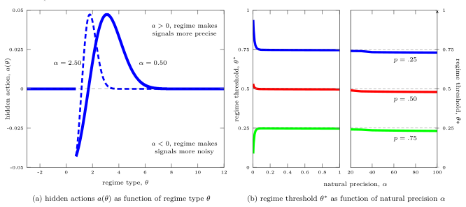
Panel (a) shows the regime’s actions to directly manipulate the number of signals \(n(a)\). For intermediate \(\theta\) it is optimal for \(a(\theta)<0\) so that the regime makes the signal more noisy than the natural precision, \(n(a(\theta))<\alpha\). For high \(\theta\) it is optimal for \(a(\theta)>0\) so that the regime clarifies its strength by making the signal more precise, \(n(a(\theta))>\alpha\). In this example the opportunity cost is \(p=.25\). Panel (b) shows \(\theta^*\) as a function of the \(\alpha\) for various \(p\). The regime benefits from information manipulation in that \(\theta^*< 1-p\) when \(\alpha\) is high enough. All calculations use the bounds \(\underline{n}=\alpha/2\), \(\overline{n}=3\alpha/2\) and cost function \(C(a)=a^2/2\).
This version of the model is somewhat less tractable than the benchmark and it is difficult to analytically characterize the regime threshold \(\theta^*\) as a function of the natural precision \(\alpha\). But it is straightforward to solve for \(\theta^*\) numerically. The right panel of Figure 4 shows \(\theta^*\) as the natural precision \(\alpha\) varies from 0 to 100. Notice that diminishing returns to information manipulation set in fast when the intrinsic \(\alpha\) is high. A five-fold increase in \(\alpha\) from \(.5\) to \(2.5\) hardly shifts the threshold \(\theta^*\) at all. Despite the lack of bias in signals, the regime can still benefit from information manipulation in this setting. For high enough \(\alpha\) we have \(\theta^*<1-p\) so that again information manipulation is effective (see Appendix A for more details).
Discussion. This example shows that the regime can benefit from information manipulation even if it is not able to introduce bias. Edmond (2012) provides a related example, developing a model where citizens and the regime have quadratic preferences of the kind used in the cheap-talk literature and showing that while citizens in this setting can infer the bias in their information (and so there is no bias in equilibrium), their signals are endogenously noisier in a way that helps the regime prevent coordination against its interests.
The variation in the regime’s preferences over the number of signals is reminiscent of results on information provision by a monopolist, as in Lewis and Sappington (1991, 1994) or Johnson and Myatt (2006). In Johnson and Myatt (2006) for example, a monopolist’s preferences over the posterior precision of consumer beliefs about a product depends on the amount of prior dispersion in beliefs; a monopolist facing a homogeneous population deploys a mass-market, low-markup strategy and keeps information low, but a monopolist facing a more heterogeneous population deploys a more niche, high-markup strategy and provides more information. In models of this kind, however, the private information lies on the consumers’ side rather than the monopolist’s and the ex post information provision (if any) is observable by consumers. In my model, by contrast, the ex post information provision varies with the regime’s unobservable type and citizens have to make inferences about the endogenous precision of their information jointly with their inferences about the type itself.
6.2 Struggles over Information
I now return to the setting of shifts in the signal mean with exogenous signal precision. I suppose however that there is an opposition and that if a regime is of type \(\theta\) and takes action \(a\) while the opposition takes action \(e\), then citizens have signals \(x_i = \theta + a - e + \varepsilon_i\) where \(\varepsilon_i\) is IID normal with mean zero and precision \(\alpha\). The regime’s action \(a\) increases the signal mean while the opposition’s action \(e\) decreases it. Both actions are unobserved by citizens.
To highlight the struggle over manipulating information, I assume that the regime and the opposition both know the regime’s type \(\theta\). Along the equilibrium path citizens receive signals with mean \(\theta+a(\theta)-e(\theta)\). If \(a(\theta)=e(\theta)\), then the opposition simply undoes the efforts of the regime. I assume the regime has strictly convex cost \(C(a)\) with \(C'(0)=0\) and the opposition has cost \(C(\kappa e)/\kappa\) for some parameter \(\kappa>0\). If \(\kappa>1\) the regime has a cost advantage.
The payoff to the opposition is of the form \(S-C(\kappa e)/\kappa\), so the opposition prefers the attack to be as large as possible, similar to the dissidents in Bueno de Mesquita (2010). Taking the aggregate attack \(S(\theta,a,e)\) as given, an equilibrium in the subgame between the regime and the opposition consists of hidden actions \(a(\theta),e(\theta)\) that are mutual best responses \begin{align} a(\theta)&\in \operatornamewithlimits{argmax}_{a\geq0}\left\{B(\theta,S(\theta,a,e(\theta)))-C(a) \right\}\\ e(\theta)&\in \operatornamewithlimits{argmax}_{e\geq0}\left\{S(\theta,a(\theta),e) - C(\kappa e)/\kappa \right \} \tag{32}\end{align} The regime’s outside option introduces a key asymmetry. The regime does not care about the size of \(S\) in those states where it is overthrown. By contrast, the opposition cares about \(S\) both when the regime is overthrown and when it is not.
I again restrict attention to a monotone equilibrium where citizens participate if their signal is \(x_i<x^*\) and the regime is overthrown if \(\theta<\theta^*\), for thresholds \(x^*,\theta^*\) to be determined. The main result here is:
Proposition 8. Conditional on the regime’s survival, \(\theta\geq\theta^*\), the regime and opposition actions are proportional, \(a(\theta)=\kappa e(\theta)\). Moreover, if the signal precision \(\alpha\) is sufficiently high, then the regime threshold \(\theta^*\) is strictly less than the Morris-Shin benchmark \(\theta^*_{\text{MS}}=1-p\), despite the opposition.
In a monotone equilibrium the aggregate attack is \(S(\theta,a,e)=\Phi(\sqrt{\alpha}(x^*-\theta-a+e))\). The first order condition for the regime is \(C'(a)=\sqrt{\alpha}\phi(\sqrt{\alpha}(x^*-\theta-a+e(\theta)))\) for \(\theta\geq\theta^*\) while the first order condition for the opposition is \(C'(\kappa e)=\sqrt{\alpha}\phi(\sqrt{\alpha}(x^*-\theta-a(\theta)+e))\). Thus if the regime survives, \(\theta\geq\theta^*\), then along the equilibrium path the marginal benefit of manipulation is the same for both the regime and the opposition and the level of manipulation is simply determined by their respective marginal costs \(C'(a(\theta))=C'(\kappa e(\theta))\) so that \(a(\theta) = \kappa e(\theta)\) (since \(C(\cdot)\) is strictly convex). In short, when the regime survives its actions are larger than those of the opposition if and only if the regime has a cost advantage, \(\kappa>1\).
The left panel of Figure 5 illustrates, with \(\kappa>1\) so that the regime’s actions \(a(\theta)\) are larger than the opposition’s actions \(e(\theta)\) on \(\theta\geq\theta^*\). Just as the regime’s hidden actions jump discretely to \(a(\theta^*)>0\) at the threshold \(\theta=\theta^*\), so too do the opposition’s actions typically jump at the threshold (though their jump may be up or down, depending on parameters). For \(\theta<\theta^*\) only the opposition takes any action.
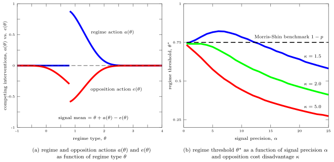
Panel (a) shows the regime’s and opposition’s actions \(a(\theta)\) and \(e(\theta)\) when there is a struggle over information. For clarity the opposition’s \(e(\theta)\) is plotted on a negative scale. For \(\theta<\theta^*\), only the opposition takes an action. For \(\theta\geq\theta^*\) the actions satisfy \(a(\theta)=\kappa e(\theta)\), where \(\kappa\) measures the costliness of the opposition’s action. In this example, \(\kappa=1.5\) and the opposition’s costs are greater than the regime’s. Panel (b) shows \(\theta^*\) as a function of the signal precision \(\alpha\) for various \(\kappa\). In these examples, the regime still benefits from information manipulation in that \(\theta^*< 1-p\) when \(\alpha\) is high enough. In these calculations, the opportunity cost is \(p=.25\) and the regime’s cost function is \(C(a)=a^2/2\) so that the opposition’s cost function is \(\kappa e^2/2\).
Does the presence of an opposition change the effectiveness of a regime’s manipulation? On the one hand, it is true that the presence of the opposition generally moves the threshold \(\theta^*\) against the regime (it is higher than it would be in the model where there is no opposition, \(\kappa=\infty\)). On the other hand, the regime still manipulates information and for high enough signal precision \(\alpha\) the regime threshold \(\theta^*\) is less than the Morris-Shin benchmark \(\theta^*_{\text{MS}}=1-p\), just as in the benchmark model. The right panel of Figure 5 illustrates, showing the effects of changing \(\alpha\) for various levels of \(\kappa\). Not surprisingly, when \(\kappa\) is relatively high, so that the opposition is at a pronounced disadvantage, it takes only a small increase in \(\alpha\) for the regime’s manipulation to be effective.
These results suggest that while the presence of organized opposition is important for understanding how much manipulation takes place and for the equilibrium level of the regime threshold \(\theta^*\), it is less important for the result that the regime threshold can be decreasing in the signal precision so that more precise signals move the threshold in the regime’s favor.
7 Conclusions
I develop a signal-jamming model of information and political regime change. In contrast with familiar signal-jamming models, the regime’s manipulation presents citizens with a difficult signal-extraction problem and the manipulation is often payoff improving for the regime. The model predicts that (i) holding fixed the number of signals available to citizens, an increase in the per-unit precision of individual signals can make signal-jamming more effective and thereby make the regime harder to overthrow, but (ii) an increase in the number of signals, which simultaneously increases both the total signal precision and the regime’s costs of information manipulation, instead makes the regime easier to overthrow — unless there are strong economies of scale in information control.
The model thus allows for two kinds of information revolutions. In the first kind, perhaps best associated with the role of mass media propaganda under the totalitarian regimes of the early twentieth century, an information revolution consists of many high precision sources of information but these technologies are more centralized and subject to strong economies of scale. By establishing a large fixed propaganda apparatus, the regime can then control additional newspapers, radio stations, cinemas, etc at low marginal cost. This kind of information revolution is favorable to a regime’s survival prospects. In the second kind, perhaps best associated with the rise of social media and other more decentralized sources of information, however, there are less likely to be strong economies of scale in information control. This kind of information revolution is unfavorable to a regime’s survival prospects.
The coordination game studied in this paper is deliberately stylized so as to focus attention on the effectiveness of the regime’s manipulation and its sensitivity to changes in the information environment. For example, the model takes as given the degree of influence the regime has over citizens’ sources of information. It would clearly be interesting to develop a richer model where the degree of influence over the media is itself an equilibrium outcome, in the spirit of Besley and Prat (2006) or Gehlbach and Sonin (2008), that needs to be determined jointly with the regime’s manipulation and survival probability.
At a more general level, this paper concerns a policy-maker seeking to induce information receivers to coordinate on the policy-maker’s preferred outcome. Similar issues are likely to be at work in many scenarios. For example, the managers of a bank may try to influence information to prevent a run on deposits. But in market-oriented scenarios (such as a bank run, or a currency crisis), market prices are also likely to aggregate information and may interact with the policy-maker’s actions in complicated ways (cf., Angeletos and Werning 2006; Hellwig et al. 2006). In that sense, the analysis in this paper should be viewed as suggestive of a key element that would be operative in a more complete, but also more complex, account of information manipulation in market-oriented coordination games.
A Proofs and Omitted Derivations
A.1 Morris-Shin Benchmark
Let \(\hat{x},\hat{\theta}\) denote candidates for the critical thresholds. The posterior beliefs of a citizen with \(x_i\) facing \(\hat{\theta}\) are given by \(\text{Prob}[\theta < \hat{\theta}\,|\,x_i]=\Phi(\sqrt{\alpha }(\hat{\theta}-x_i))\). A citizen with \(x_i\) will participate if and only if \(\Phi(\sqrt{\alpha }(\hat{\theta}-x_i))\geq p\). This probability is continuous and strictly decreasing in \(x_i\), so for each \(\hat{\theta}\) there is a unique signal for which a citizen is indifferent. Similarly, if the regime faces threshold \(\hat{x}\) the aggregate attack is \(\text{Prob}[x_i<\hat{x}\,|\,\theta]=\Phi(\sqrt{\alpha }(\hat{x}-\theta ))\). A regime \(\theta\) will not be overthrown if and only if \(\theta \geq \Phi (\sqrt{\alpha }(\hat{x}-\theta))\). The probability on the right hand side is continuous and strictly decreasing in \(\theta\), so for each \(\hat{x}\) there is a unique regime type that is indifferent. The Morris-Shin thresholds \(x_{\text{MS}}^{*},\theta _{\text{MS}}^{*}\) simultaneously solve these best response conditions as equalities, as stated in equations (4)-(5) in the main text. It is then straightforward to verify that there is only one solution to these equations and that \(\theta^*_{\text{MS}}=1-p\) independent of \(\alpha\) and \(x^*_{\text{MS}}=1-p-\Phi^{-1}(p)/\sqrt{\alpha}\).
A.2 Proof of Proposition 1
The proof shows first that (i) there is a unique equilibrium in monotone strategies, and (ii) that the unique monotone equilibrium is the only equilibrium which survives the iterative elimination of interim strictly dominated strategies. For ease of exposition, the proof is broken down into separate lemmas.
(i) Unique equilibrium in monotone strategies
Regime problem. Let \(\hat{x}\in\mathbb{R}\) denote a candidate for the citizens’ threshold.
Lemma 1. For each \(\hat{x}\in\mathbb{R}\), the unique solution to the regime’s decision problem is characterized by a pair of functions, \(\Theta:\mathbb{R}\rightarrow[0,1)\) and \(A:\mathbb{R}\rightarrow\mathbb{R}_+\) such that if citizens participate for all \(x_i<\hat{x}\) then the best-response of the regime is to abandon if and only if its type is \(\theta<\Theta(\hat{x})\) and to choose an action \(a(\theta)=0\) for \(\theta<\Theta(\hat{x})\) and \(a(\theta)=A(\theta-\hat{x})\) for \(\theta\geq\Theta(\hat{x})\).
Proof of Lemma 1. To begin, let \[\tag{33} S(w):= \Phi(-\sqrt{\alpha}w)\] The auxiliary function \(S(w)\) is exogenous and does not depend on \(\hat{x}\). In terms of this function, the aggregate attack facing the regime is \[\tag{34} \int_{-\infty}^{\hat{x}}\sqrt{\alpha}\phi(\sqrt{\alpha}(x_i-\theta-a))\,dx_i = \Phi(\sqrt{\alpha}(\hat{x}-\theta-a))=S(\theta+a-\hat{x})\] Since the regime has access to an outside option normalized to zero, its problem can be written \[\tag{35} V(\theta,\hat{x}) := \max[0,W(\theta,\hat{x})]\] where \(W(\theta,\hat{x})\) is the best payoff regime \(\theta\) can get if it is not overthrown \[\tag{36} W(\theta,\hat{x}) := \max_{a\geq 0} \left[\theta-S(\theta+a-\hat{x})-C(a)\right]\] From the envelope theorem, the partial derivative \(W_{\theta}(\theta,\hat{x}) = 1-S'(\theta-\hat{x}+a)>1\) since \(S'(w)<0\) for all \(w\in\mathbb{R}\). Since \(S(w)\geq0\) and \(C(a)\geq0\) we know \(W(\theta,\hat{x})<0\) for all \(\theta<0\) and all \(\hat{x}\). Similarly, \(W(1,\hat{x})>0\) for all \(\hat{x}\). So by the intermediate value theorem there is a unique \(\Theta(\hat{x})\in[0,1)\) such that \(W(\Theta(\hat{x}),\hat{x})=0\). And since \(W_{\theta}(\theta,\hat{x})>1\) the regime is overthrown if and only if \(\theta<\Theta(\hat{x})\). Since positive actions are costly, the regime takes no action for \(\theta<\Theta(\hat{x})\). Otherwise, for \(\theta\geq\Theta(\hat{x})\), the actions of the regime are given by \[\tag{37} a(\theta) = A(\theta-\hat{x})\] where the function \(A(t)\) is exogenous and does not depend on \(\hat{x}\). This auxiliary function is defined by: \[\tag{38} A(t):=\operatornamewithlimits{argmin}_{a\geq 0} \left[S(t+a) + C(a)\right]\] The first order necessary condition for interior solutions can be written \(C'(a)=-S'(t+a)\), and, on using the formula for \(S(\cdot)\) in equation (33) above, \(C'(a) = \sqrt{\alpha}\phi(\sqrt{\alpha}(t+a))\) where \(\phi(w):=\exp(-w^2/2)/\sqrt{2\pi}\) for all \(w\in\mathbb{R}\). This first order condition may have zero, one or two solutions for each \(t\). If for a given \(t\) there are zero (interior) solutions, then \(A(t)=0\). If for given \(t\) there are two solutions, one of them can be ruled out by the second order sufficient condition \(\alpha\phi'(\sqrt{\alpha}(t+a))+C''(a)>0\). Using the property \(\phi'(w)=-w\phi(w)\) for all \(w\in\mathbb{R}\) shows that if there are two solutions to the first order condition, only the “higher” of them satisfies the second order condition. Therefore for each \(t\) there is a single \(A(t)\) that solves the regime’s problem. Making the substitution \(t=\theta-\hat{x}\), the regime’s threshold \(\Theta(\hat{x})\) is then found from the indifference condition \(W(\Theta(\hat{x}),\hat{x})=0\), or more explicitly \[\tag{39} \Theta(\hat{x})=S(\Theta(\hat{x})-\hat{x}+A(\Theta(\hat{x})-\hat{x}))+C(A(\Theta(\hat{x})-\hat{x})))\] Taking \(\hat{x}\) as given, equations (38) and (39) give the regime threshold \(\Theta(\hat{x})\) and the hidden actions \(a(\theta)=A(\theta-\hat{x})\) that solve the regime’s problem.\(\hfill\square\)
Citizen problem. Let \(\hat{\theta}\in[0,1)\) and \(a:\mathbb{R}\rightarrow\mathbb{R}_+\) denote, respectively, a candidate for the regime’s threshold and a candidate for the regime’s hidden actions with \(a(\theta)=0\) for \(\theta<\hat{\theta}\).
Lemma 2. For each \(\hat{\theta}\in[0,1)\) and \(a:\mathbb{R}\rightarrow\mathbb{R}_+\)
The unique solution to the problem of a citizen with signal \(x_i\) is given by a mapping \(P(\cdot\,|\,a(\cdot)):\mathbb{R}\times\mathbb{R}\rightarrow[0,1]\) such that the citizen participates if and only if \[\tag{40} P(x_i,\hat{\theta}\,|\,a(\cdot)) := \text{Prob}[\theta<\hat{\theta}\;|\;x_i,a(\cdot)]\geq p\] where \(P\) is continuous and strictly decreasing in \(x_i\) with limits \(P(-\infty,\hat{\theta}\,|\,a(\cdot))=1\) and \(P(+\infty,\hat{\theta}\,|\,a(\cdot)))=0\) for any \(\hat{\theta}\) and function \(a(\cdot)\) satisfying \(a(\theta)=0\) for \(\theta<\hat{\theta}\).
For any candidate citizen threshold \(\hat{x}\), with implied regime threshold \(\Theta(\hat{x})\) and hidden actions \(A(\theta-\hat{x})\), an individual citizen with signal \(x_i\) participates if and only if its signal is such that \[\tag{41} K(x_i,\hat{x}) := \text{Prob}[\theta<\Theta(\hat{x})\;|\;x_i,A(\cdot)] \geq p\] where \(K:\mathbb{R}\times\mathbb{R}\rightarrow[0,1]\) is continuous, strictly increasing in \(x_i\) with limits \(K(-\infty,\hat{x})=0\) and \(K(+\infty,\hat{x})=1\) for any \(\hat{x}\). Moreover, \(K(x_i,\hat{x}) = \text{Prob}[\theta<\Theta(\hat{x})-\hat{x}\;|\;x_i-\hat{x},A(\cdot)]\) for any \(\hat{x}\).
Proof of Lemma 2. (a) For notational simplicity, write \(x\) for an individual’s signal, \(\theta\) for the regime threshold, and \(P(x,\theta)\) for the probability an individual with \(x\) assigns to the regime’s type being less than \(\theta\) when the actions are \(a:\mathbb{R}\rightarrow\mathbb{R}_+\). That is,
\[\tag{42} P(x,\theta)= \frac{\int_{-\infty}^{\theta}\sqrt{\alpha }\phi (\sqrt{\alpha }(x_i-t))\,dt }{\int_{-\infty }^{\infty }\sqrt{\alpha }\phi (\sqrt{\alpha }(x_i-t -a(t)))\,dt }\] where the numerator uses \(a(t)=0\) for \(t<\theta\). Hence \(P:\mathbb{R}\times\mathbb{R}\rightarrow[0,1]\) is continuous in \(x,\theta\). This probability can be written \[\tag{43} P(x,\theta)=\frac{N(\theta-x)}{N(\theta-x)+D(x,\theta)}\] where \[\tag{44} N(\theta-x):=\Phi(\sqrt{\alpha}(\theta-x)),\quad \text{and} \quad D(x,\theta):=\int_{\theta}^{\infty }\sqrt{\alpha }\phi (\sqrt{\alpha }(x-\xi -a(\xi)))\,d\xi\] Differentiating (43) shows \(P_x <0\) if and only if \(N'/N>-D_{x}/D\). Calculating the derivatives shows that this is equivalent to \[\tag{45} H(\sqrt{\alpha}(x - \theta)) > -\frac{\int_{\theta}^{\infty}\phi'(\sqrt{\alpha}(x-y(\xi)))\,d\xi}{\int_{\theta}^{\infty}\phi(\sqrt{\alpha}(x-y(\xi)))\,d\xi} = \frac{\int_{\theta}^{\infty}\sqrt{\alpha}(x-y(\xi))\phi(\sqrt{\alpha}(x-y(\xi)))\,d\xi}{\int_{\theta}^{\infty}\phi(\sqrt{\alpha}(x-y(\xi)))\,d\xi}\] where \(H(w):=\phi(w)/(1-\Phi(w))>0\) denotes the standard normal hazard function for \(w\in\mathbb{R}\), where \(y(\xi):=\xi+a(\xi)\) is the mean of the signal distribution if \(\xi\geq\theta\), and where the equality follows from \(\phi'(w)=-w\phi(w)\) for all \(w\). Now define a density \(\varphi(\xi\,|\,x)>0\) by \[\tag{46} \varphi(\xi\,|\,x):=\frac{\phi(\sqrt{\alpha}(x-y(\xi)))}{\int_{\theta}^{\infty}\phi(\sqrt{\alpha}(x-y(\xi')))\,d\xi'},\qquad \xi\in[\theta,\infty)\] Then after a slight rearrangement of terms in (45), \(P_x<0\) if and only if \[\tag{47} H(\sqrt{\alpha}(x-\theta)) - \sqrt{\alpha}(x - \theta) > \sqrt{\alpha}\left[\theta - \int_{\theta}^{\infty}y(\xi)\varphi(\xi\,|\,x)\,d\xi\right]\] Since the hazard function satisfies \(H(w)>w\) for all \(w\in\mathbb{R}\) and \(\alpha>0\), it is sufficient that \[\tag{48} \int_{\theta}^{\infty}y(\xi)\varphi(\xi\,|\,x)\,d\xi \geq \theta\] But since \(y(\xi):=\xi+a(\xi)\), \(\xi\geq\theta\), and \(a(\xi)\geq0\), condition (48) is always satisfied. Therefore \(P_x<0\). Since \(N'>0\) and \(D_{\theta}<0\), \(P_{\theta}>0\) for all \(x,\theta\). Moreover, since \(N(-\infty)=0\) and \(D>0\) we have \(P(x,-\infty)=0\) for all \(x\). Similarly, since \(a(\xi)=0\) for all \(\xi<\theta\) as \(\theta\rightarrow\infty\) we have \(D(x,\theta)\rightarrow 1-N(\theta-x)\) and since \(N(+\infty)=1\) this means \(D(x,+\infty)=0\) for all \(x\). Therefore \(P(x,+\infty)=1\) for all \(x\). The limit properties in \(x\) are established in parallel fashion.
(b) Fix a \(\hat{x}\in\mathbb{R}\) and let \(A(\theta-\hat{x})\) denote the associated hidden actions. Analogous to (43), write \(P(x,\theta,\hat{x}) = N(\theta-x)/[N(\theta-x)+D(x,\theta,\hat{x})\) where \(N:\mathbb{R}\rightarrow[0,1]\) is defined as in (44) above and where \[\tag{49} D(x,\theta,\hat{x}) := \int_{\theta}^{\infty }\sqrt{\alpha }\phi (\sqrt{\alpha }(x-t -A(t-\hat{x})))\,dt\] Now define \(K(x,\hat{x}):=P(x,\Theta(\hat{x}),\hat{x})\). That \(K(x,\hat{x})\) is continuous and decreasing in \(x\) is immediate from part (a) above. Finally, for \(K(x,\hat{x}) = P(x-\hat{x},\Theta(\hat{x})-\hat{x},0)\) it is sufficient that \(D(x,\Theta(\hat{x}),\hat{x})=D(x-\hat{x},\Theta(\hat{x})-\hat{x},0)\). From (49) and using the change of variables \(\xi:=\theta-\hat{x}\) we have \[\tag{50} D(x,\Theta(\hat{x}),\hat{x}) = \int_{\Theta(\hat{x})-\hat{x}}^{\infty }\sqrt{\alpha }\phi (\sqrt{\alpha }(x-\hat{x}-\xi -a(\xi)))\,d\xi =D(x-\hat{x},\Theta(\hat{x})-\hat{x},,0)\] Therefore \(K(x,\hat{x}) = P(x-\hat{x},\Theta(\hat{x})-\hat{x},0)=\text{Prob}[\theta<\Theta(\hat{x})-\hat{x}\;|\;x-\hat{x},A(\cdot)]\) as claimed.\(\hfill\square\)
Fixed point. A citizen with signal \(x_i\) will participate if and only if \(K(x_i,\hat{x})\geq p\). Since \(K(x_i,\hat{x})\) is strictly increasing in \(x_i\) with \(K(-\infty,\hat{x})<p\) and \(K(+\infty,\hat{x})>p\) for any \(\hat{x}\in\mathbb{R}\), there is a unique signal \(\psi(\hat{x})\) solving \[\tag{51} K(\psi(\hat{x}),\hat{x}) = p\] such that a citizen with signal \(x_i\) participates if and only if \(x_i<\psi(\hat{x})\).
Lemma 3. The function \(\psi:\mathbb{R}\rightarrow\mathbb{R}\) is continuous and has a unique fixed point \(x^*=\psi(x^*)\) with derivative \(\psi'(x^*)\in(0,1)\) at the fixed point. Moreover \(\psi(x)\leq x^*\) for all \(x<x^*\) and \(\psi(x)\geq x^*\) for all \(x>x^*\).
Proof of Lemma 3. Since \(K(x,\hat{x})\) is continuously differentiable in \(x\), an application of the implicit function theorem to (51) shows that \(\psi(\cdot)\) is continuous. Fixed points of \(\psi(\cdot)\) satisfy \(x^*=\psi(x^*)\). Equivalently, by part (b) of Lemma 2, they satisfy \(K(x^*,x^*)=P(0,\Theta(x^*)-x^*,0)=p\), where \(\Theta(\hat{x})\) is the critical state in the regime’s problem (38)-(39). By Lemma 2 and the intermediate value theorem there is a unique \(z^*\in\mathbb{R}\) such that \(P(0,z^*,0)=p\). Then applying the implicit function theorem to (38)-(39) gives \[\tag{52} \Theta'(\hat{x}) = \frac{\sqrt{\alpha}\phi(\sqrt{\alpha}(\hat{x}-\Theta(\hat{x})-A(\Theta(\hat{x})-\hat{x})))}{1+\sqrt{\alpha}\phi(\sqrt{\alpha}(\hat{x}-\Theta(\hat{x})-A(\Theta(\hat{x})-\hat{x})))}\in(0,1)\] Since \(\Theta(-\infty)=0\) and \(\Theta(+\infty)=1\), there is a unique \(x^*\in\mathbb{R}\) such that \(\Theta(x^*)-x^*=z^*\), hence \(\psi(\cdot)\) has a unique fixed point, the same \(x^*\). Now using part (b) of Lemma 2 and implicitly differentiating (51) we have \[\tag{53} \psi'(\hat{x}) = 1 + \frac{P_{\theta}(\psi(\hat{x})-\hat{x},\Theta(\hat{x})-\hat{x},0)}{P_x (\psi(\hat{x})-\hat{x},\Theta(\hat{x})-\hat{x},0)} (1-\Theta'(\hat{x}))\] By Lemma 2, \(P_{\theta}>0\) and \(P_x <0\) and \(\Theta'(\hat{x})\in(0,1)\) from (52). Therefore \(\psi'(\hat{x})<1\) for all \(\hat{x}\). To see that \(\psi'(x^*)>0\), first notice that it is sufficient that \(P_{\theta}/P_x \geq-1\) when evaluated at \(\hat{x}=x^*\). Calculating the derivatives shows that this is true if and only if \[\tag{54} \phi(\sqrt{\alpha}(y(\theta^*)-x^*)) + \int_{\theta^*}^{\infty}\sqrt{\alpha}\phi'(\sqrt{\alpha}(y(\theta)-x^*))\,d\theta\leq0\] where \(\theta^*:=\Theta(x^*)\) and where \(y(\theta)=\theta+a(\theta)\) is the mean of the signal distribution from which a citizen is sampling if the regime has type \(\theta\geq\theta^*\). To show that this condition always holds, we need to consider the cases of linear costs and strictly convex costs separately. If costs are linear, \(C(a)=ca\), then if \(c\geq\overline{c}:=\sqrt{\alpha}\phi(0)\) the result is trivial because \(a(\theta)=0\) for all \(\theta\in\mathbb{R}\). So suppose \(c<\overline{c}\). Then \(a(\theta)=\max[0,x^*+\gamma-\theta]\) where \(\gamma := \sqrt{2\log\left(\sqrt{\alpha}\phi(0)/c\right)/\alpha}>0\). Calculating the integral and then simplifying shows that (54) holds if and only if \(-\alpha\gamma\phi(\sqrt{\alpha}\gamma)a(\theta^*)\leq0\) which is true because \(a(\theta^*)\geq0\). If costs are strictly convex, then from the optimality conditions for the regime’s choice of action we have that \(a(\theta)>0\) for all \(\theta\geq\theta^*\) and \[\tag{55} \sqrt{\alpha}\phi(\sqrt{\alpha}(y(\theta)-x^*)) = C'(a(\theta)),\quad \theta\geq\theta^*\] Differentiating with respect to \(\theta\) gives \[\tag{56} \alpha \phi'(\sqrt{\alpha}(y(\theta)-x^*))y'(\theta) = C''(a(\theta))a'(\theta),\quad \theta\geq\theta^*\] Using the associated second order condition shows that \(y'(\theta)>0\) for \(\theta\geq\theta^*\). Since \(y(\cdot)\) is invertible, a change of variables shows that (54) holds if and only if \[\tag{57} \int_{\theta^*}^{\infty}\phi'(\sqrt{\alpha}(y(\theta)-x^*)) \frac{a'(\theta)}{y'(\theta)}\,d\theta \geq0\] Using (56) we equivalently have the condition \[\tag{58} \int_{\theta^*}^{\infty}\frac{\phi'(\sqrt{\alpha}(y(\theta)-x^*))^2}{C''(a(\theta))}\, d\theta \geq 0\] which is true since the integrand is non-negative. Therefore, \(P_{\theta}/P_x\geq-1\) at \(\hat{x}=x^*\) and \(\psi'(x^*)>0\).
Finally, \(\psi(\hat{x})\leq x^*\) for every \(\hat{x}<x^*\) is proven by contradiction. Suppose not. Then by continuity of \(\psi\) there exists \(\tilde{x}<x^*\) such that \(\psi(\tilde{x})=x^*\). Moreover, since \(\psi'(x^*)>0\), we must have \(\psi'(\tilde{x})<0\) for at least one such \(\tilde{x}\). Since \(\psi(\tilde{x})=x^*\) and \(K(x^*,x^*)=p\), under this hypothesis we can write \(K(\psi(\tilde{x}),\psi(\tilde{x}))=p\) so by the implicit function theorem \(\psi(\tilde{x})\) must satisfy \[\tag{59} \psi'(\tilde{x})[K_1(x^*,x^*)+K_2(x^*,x^*)]=0\] where the hypothesis \(\psi(\tilde{x})=x^*\) is used to evaluate the partial derivatives \(K_1\) and \(K_2\). Since \(\psi'(\tilde{x})<0\), this can only be satisfied if \(K_1(x^*,x^*)+K_2(x^*,x^*)=0\). But for any \(\hat{x}\in\mathbb{R}\), the value \(\psi(\hat{x})\) is implicitly defined by \(K(\psi(\hat{x}),\hat{x})=p\) so that by the implicit function theorem \(\psi'(\hat{x}) = -K_2(\psi(\hat{x}),\hat{x})/K_1(\psi(\hat{x}),\hat{x})\). From (53) we know \(\psi'(\hat{x})<1\) for any \(\hat{x}\) and since \(K_1<0\) from Lemma 2 we conclude \(K_1(\psi(\hat{x}),\hat{x})+K_2(\psi(\hat{x}),\hat{x})<0\) for any \(\hat{x}\). For \(\hat{x}=x^*\) in particular, \(K_1(x^*,x^*)+K_2(x^*,x^*)<0\) so we have the needed contradiction. Therefore \(\psi(\hat{x})\leq x^*\) for every \(\hat{x}<x^*\). A symmetric argument shows \(\psi(\hat{x})\geq x^*\) for every \(\hat{x}>x^*\). \(\hfill\square\)
Concluding that there is a unique equilibrium in monotone strategies. To conclude part (i) of the proof, we take an arbitrary \(\hat{x}\in\mathbb{R}\) and solve the regime’s problem to get \(\Theta(\hat{x})\) and \(a(\theta,\hat{x})=A(\theta-\hat{x})\) using the auxiliary function from Lemma 1. We use these functions to construct \(K(x_i,\hat{x})\) from (41) for each signal \(x_i\in\mathbb{R}\) and use Lemma 2 to conclude that in particular \(K(\hat{x},\hat{x})=P(0,\Theta(\hat{x})-\hat{x},0)\). We then use the intermediate value theorem to deduce that there is a unique \(z^*\in\mathbb{R}\) such that \(P(0,z^*,0)=p\). This gives a unique difference \(z^*=\theta^*-x^*\) that can be plugged into the regime’s indifference condition (39) to get the unique \(\theta^*=\Theta(x^*)\in[0,1)\) such that the regime is overthrown if and only if \(\theta<\theta^*\). The unique signal threshold is then \(x^*=\theta^*-z^*\) and the unique hidden action function is given by \(a(\theta):=A(\theta-x^*)\).
(ii) Iterative elimination of interim strictly dominated strategies
We can now go on to show that there is no other equilibrium. The argument begins by showing that for sufficiently low signals it is a dominant strategy to participate in the attack on the regime and for sufficiently high signals it is a dominant strategy to not participate.
Dominance regions. If the regime has \(\theta<0\), any mass \(S\geq0\) can overthrow the regime. Similarly, if the regime has \(\theta\geq1\) it can never be overthrown. Any regime that is overthrown takes no action, since to do so would incur a cost for no gain. Similarly, any regime \(\theta\) that is not overthrown takes an action no larger than the \(a\) such that \(\theta=C(a)\). Any larger action must result in a negative payoff which can be improved upon by taking the outside option. Given this:
Lemma 4. There exists a pair of signals \(\underline{x}<\overline{x}\), both finite, such that \(s(x_i)=1\) is strictly dominant for \(x_i<\underline{x}\) and \(s(x_i)=0\) is strictly dominant for \(x_i>\overline{x}\).
Proof of Lemma 4. The most pessimistic scenario for any citizen is that regimes are overthrown only if \(\theta<0\) and that regimes take the largest hidden actions that could be rational \(\underline{a}(\theta):=C^{-1}(\theta)\) for \(\theta\geq0\) and zero otherwise. Let \(\underline{P}(x_i):=\text{Prob}[\theta<0\;|\;x_i,\; \underline{a}(\cdot)]\) denote the probability the regime is overthrown in this most pessimistic scenario. Part (a) of Lemma 2 holds for hidden actions of the form \(\underline{a}(\theta)\) and implies \(\underline{P}'(x_i)<0\) for all \(x_i\), and since \(\underline{P}(-\infty)=1\) and \(\underline{P}(+\infty)=0\) by the intermediate value theorem there is a unique value, \(\underline{x}\), finite, such that \(\underline{P}(\underline{x})=p\). For \(x_i<\underline{x}\) it is (iteratively) strictly dominant for \(s(x_i)=1\). Similarly, the most optimistic scenario for any citizen is that regimes are overthrown if \(\theta<1\) and that regimes take the smallest hidden actions that could be rational \(\overline{a}(\theta):=0\). Let \(\overline{P}(x_i):=\text{Prob}[\theta<1\;|\;x_i,\; \overline{a}(\cdot)]\) denote the probability the regime is overthrown in this most optimistic scenario. A parallel argument establishes the existence of a unique value, \(\overline{x}\), finite, such that \(\overline{P}(\overline{x})=p\). For \(x_i>\overline{x}\) it is (iteratively) strictly dominant for \(s(x_i)=0\). \(\hfill\square\)
Iterative elimination. Starting from the dominance regions implied by \(\underline{x}\) and \(\overline{x}\) it is then possible to iteratively eliminate (interim) strictly dominated strategies. Recall that \(S(w):= \Phi(-\sqrt{\alpha}w)\) and \(A(t) := \operatornamewithlimits{argmin}_{a\geq 0} \left[S(t+a) + C(a)\right]\). Again, these auxiliary functions do not depend on any endogenous variable and in particular do not depend on citizen thresholds.
Lemma 5. Let \(x_{n+1}=\psi(x_n)\) for \(n=0,1,2,...\) where \[ K(\psi(x_n),x_n) = p\]
If it is strictly dominant for \(s(x_i)=1\) for all \(x_i<\underline{x}_n\), then the regime is overthrown for at least all \(\theta<\underline{\theta}_n:=\Theta(\underline{x}_n)\) where the function \(\Theta:\mathbb{R}\rightarrow[0,1)\) solves \[\tag{60} \Theta(x) = S(\Theta(x)-x+A(\Theta(x)-x)) + C((\Theta(x)-x))\] Similarly, if it is strictly dominant for \(s(x_i)=0\) for all \(x_i>\overline{x}_n\), then regime is not overthrown for at least all \(\theta>\overline{\theta}_n:=\Theta(\overline{x}_n)\).
Moreover, if it is strictly dominant for \(s(x_i)=1\) for all \(x_i<\underline{x}_n\), then it is strictly dominant for \(s(x_i)=1\) for all \(x_i<\underline{x}_{n+1}=\psi(\underline{x}_n)\). Similarly, if it is strictly dominant for \(s(x_i)=0\) for all \(x_i>\overline{x}_n\), then it is strictly dominant for \(s(x_i)=0\) for all \(x_i>\overline{x}_{n+1}=\psi(\overline{x}_n)\).
Proof of Lemma 5. (a) Fix an \(\underline{x}_n\) and \(\overline{x}_n\) such that citizens with signals \(x_i<\underline{x}_n\) have \(s(x_i)=1\) and likewise citizens with signals \(x_i>\overline{x}_n\) have \(s(x_i)=0\). From Lemma 4 this can be done at least for the signals \(\underline{x},\overline{x}\) that determine the bounds of the dominance regions. All citizens with signals \(x_i<\underline{x}_n\) have \(s(x_i)=1\) so the mass of subversives is at least \(\Phi(\sqrt{\alpha}(\underline{x}_n-\theta-a))\). To acknowledge this, write the total mass of subversives \[\tag{61} \Phi(\sqrt{\alpha}(\underline{x}_n-\theta-a)) + \Delta(\theta+a)\] for some function \(\Delta:\mathbb{R}\rightarrow[0,1]\). First consider the case \(\Delta(\cdot)=0\) where only citizens with \(x_i<\underline{x}_n\) subvert the regime. From Lemma 1 there is a unique threshold \(\underline{\theta}_n:=\Theta(\underline{x}_n)\in[0,1)\) sustained by hidden actions \(a(\theta)=A(\theta-\underline{x}_n)\) solving (38)-(39) such that the regime is overthrown if \(\theta<\underline{\theta}_n = \Theta(\underline{x}_n)\). Now consider the case \(\Delta(\cdot)>0\) where some citizens with signals \(x_i\geq\underline{x}_n\) also subvert the regime. The proof that the regime is overthrown for at least all \(\theta<\Theta(\underline{x}_n)\) is by contradiction. Suppose that when \(\Delta(\cdot)>0\) regime change occurs for all \(\theta<\tilde{\theta}_n\) for some \(\tilde{\theta}_n\leq\Theta(\underline{x}_n)\). A marginal regime \(\tilde{\theta}_n\) must be indifferent between being overthrown and taking the outside option, so this threshold satisfies \(\tilde{\theta}_n=S(\tilde{\theta}_n+\tilde{a}_n-\underline{x}_n) + C(\tilde{a}_n)\) where \(\tilde{a}_n\geq0\) is the optimal action for the marginal regime \(\tilde{\theta}_n\). Then observe \[\tag{62} \begin{eqnarray} \notag \Theta(\underline{x}_n) &=& \Phi[\sqrt{\alpha}(\underline{x}_n-\Theta(\underline{x}_n)-A(\Theta(\underline{x}_n)-\underline{x}_n))] + C[A(\Theta(\underline{x}_n)-\underline{x}_n))] \\ &\leq& \Phi[\sqrt{\alpha}(\underline{x}_n-\Theta(\underline{x}_n)-a)] + C(a), \\ &<& \Phi[\sqrt{\alpha}(\underline{x}_n-\Theta(\underline{x}_n)-a)]+\Delta(\tilde{\theta}_n+\tilde{a}_n) + C(a), \qquad \text{for any $a\geq 0 $} \end{eqnarray}\] where the first inequality follows because \(A(\cdot)\) minimizes \(\Phi[\sqrt{\alpha}(\underline{x}_n-\theta-a)] + C(a)\) and where the second inequality follows from \(\Delta(\cdot)>0\). Taking \(a=\tilde{a}_n\geq0\) we then have \[\tag{63} \begin{eqnarray} \notag \Theta(\underline{x}_n) &<& \Phi[\sqrt{\alpha}(\underline{x}_n-\Theta(\underline{x}_n)-\tilde{a}_n)]+\Delta(\tilde{\theta}_n+\tilde{a}_n) + C(\tilde{a}_n) \\ &=& \Phi[\sqrt{\alpha}(\underline{x}_n-\Theta(\underline{x}_n)-\tilde{a}_n)]+\Delta(\tilde{\theta}_n+\tilde{a}_n) + C(\tilde{a}_n) \\ && \,+\, \Phi[\sqrt{\alpha}(\underline{x}_n-\tilde{\theta}_n-\tilde{a}_n)] - \Phi[\sqrt{\alpha}(\underline{x}_n-\tilde{\theta}_n-\tilde{a}_n)] \\ &=& \tilde{\theta}_n + \Phi[\sqrt{\alpha}(\underline{x}_n-\Theta(\underline{x}_n)-\tilde{a}_n)] - \Phi[\sqrt{\alpha}(\underline{x}_n-\tilde{\theta}_n-\tilde{a}_n)]\\ &\leq& \tilde{\theta}_n \end{eqnarray}\] where the last inequality follows because the hypothesis \(\tilde{\theta}_n\leq\Theta(\underline{x}_n)\) implies \(\Phi[\sqrt{\alpha}(\underline{x}_n-\tilde{\theta}_n-\tilde{a}_n)] \geq \Phi[\sqrt{\alpha}(\underline{x}_n-\Theta(\underline{x}_n)-\tilde{a}_n)]\). This is a contradiction, and so \(\tilde{\theta}_n>\Theta(\underline{x}_n)\). Therefore, the regime is overthrown for at least all \(\theta<\Theta(\underline{x}_n)\). A parallel argument shows that if it is strictly dominant for \(s(x_i)=0\) for all \(x_i>\overline{x}_n\), then the regime is not overthrown for at least all \(\theta>\overline{\theta}_n:=\Theta(\overline{x}_n)\).
(b) Since cumulative distribution functions are non-decreasing, for any beliefs of the citizens, the posterior probability assigned by a citizen with signal \(x_i\) to the regime’s overthrow is at least as much as the probability they assign to \(\theta < \Theta(\underline{x}_n)\). Equivalently, \(K(x_i,\underline{x}_n)-p\) is the most conservative estimate of the expected gain to subverting. From Lemma 2 and the intermediate value theorem, there is a unique \(\underline{x}_{n+1}=\psi(\underline{x}_n)\) solving \(K(\psi(\underline{x}_n),\underline{x}_n)=p\) such that if it is strictly dominant for \(s(x_i)=1\) for all \(x_i<\underline{x}_n\), then it is strictly dominant for \(s(x_i)=1\) for all \(x_i<\underline{x}_{n}\). Similarly, there is a unique \(\overline{x}_{n+1}=\psi(\overline{x}_n)\) solving \(K(\psi(\overline{x}_n),\overline{x}_n)=p\) such that if it is strictly dominant for \(s(x_i)=0\) for all \(x_i>\overline{x}_n\), then it is strictly dominant for \(s(x_i)=0\) for all \(x_i>\overline{x}_{n+1}\). Applying the proof of part (a) at each step then completes the argument. \(\hfill\square\)
Concluding that there is no other equilibrium. Let \(\underline{x}_0 := \underline{x}\) and \(\overline{x}_0 := \overline{x}\) and generate sequences \(\{\underline{x}_n\}_{n=0}^{\infty}\) from \(\underline{x}_{n+1}=\psi(\underline{x}_n)\) and \(\{\overline{x}_n\}_{n=0}^{\infty}\) from \(\overline{x}_{n+1}=\psi(\overline{x}_n)\) where \[\tag{64} K(\psi(\overline{x}_n),\overline{x}_n) = p\] and \[\tag{65} K(\psi(\underline{x}_n),\underline{x}_n) = p\]
Part (a) of Lemma 5 maps the sequences of citizen thresholds \(\{\underline{x}_n\}_{n=0}^{\infty}\) and \(\{\overline{x}_n\}_{n=0}^{\infty}\) into monotone sequences of regime thresholds, \(\{\underline{\theta}_n\}_{n=0}^{\infty}\) from \(\underline{\theta}_n :=\Theta(\underline{x}_n)\) and \(\{\overline{\theta}_n\}_{n=0}^{\infty}\) from \(\overline{\theta}_n :=\Theta(\overline{x}_n)\). Moreover, by Lemma 3 the function \(\psi(\cdot)\) generating the sequences \(x_{n+1}=\psi(x_n)\) is continuous, has a unique fixed point \(x^*=\psi(x^*)\) with derivative \(\psi'(x^*)\in(0,1)\) at this fixed point and upper bound \(\psi(\underline{x}_n)\leq x^*\) for all \(\underline{x}_n<x^*\). From below, the sequence \(\{\underline{x}_n\}_{n=0}^{\infty}\) is bounded above, strictly monotone increasing and so converges \(\underline{x}_n \nearrow x^*\) as \(n\rightarrow\infty\). Similarly the sequence \(\{\underline{\theta}_n\}_{n=0}^{\infty}\) is bounded above, strictly monotone increasing and so converges \(\underline{\theta}_n \nearrow \theta^*=:\Theta(x^*)\) as \(n\rightarrow\infty\). From above, symmetrically, the sequence \(\{\overline{x}_n\}_{n=0}^{\infty}\) is bounded below, strictly monotone decreasing and so converges \(\overline{x}_n \searrow x^*\) as \(n\rightarrow\infty\). Similarly the sequence \(\{\overline{\theta}_n\}_{n=0}^{\infty}\) is bounded below, strictly monotone decreasing and so converges \(\overline{\theta}_n \searrow \theta^*=:\Theta(x^*)\) as \(n\rightarrow\infty\). After a finite \(n\) iterations, the only candidates for a citizen’s equilibrium strategy all have \(s(x_i)=1\) for \(x_i<\underline{x}_n\) and \(s(x_i)=0\) for \(x_i>\overline{x}_n\) with \(s(x_i)\) arbitrary for \(x_i\in[\underline{x}_n,\overline{x}_n]\). Similarly, the only candidate for the regime’s strategy has the regime abandoning for all \(\theta<\underline{\theta}_n\), not abandoning for \(\theta\geq\underline{\theta}_n\) with arbitrary choices for \(\theta\in[\underline{\theta}_n,\overline{\theta}_n]\). At each iteration, these regime thresholds are implicitly determined by hidden actions \(\underline{a}_n(\theta):=A(\theta-\underline{x}_n)\) and \(\overline{a}_n(\theta):=A(\theta-\overline{x}_n)\) respectively. In the limit as \(n\rightarrow\infty\), the only strategy that survives the elimination of strictly dominated strategies is the one with \(s(x_i)=1\) for \(x_i<x^*\) and \(s(x_i)=0\) otherwise for citizens, with the regime abandoning for \(\theta<\theta^*=\Theta(x^*)\) and hidden actions given by \(a(\theta)=A(\theta-x^*)\). Therefore the only equilibrium is the unique monotone equilibrium.\(\hfill\blacksquare\)
A.3 Proof of Proposition 2
Since the regime benefit function \(B(\theta,S)\) satisfies the Spence-Mirrlees sorting condition we have, for any \(\theta\geq\theta'\) and any \(S\geq S'\), that \[\tag{64} B(\theta,S')-B(\theta,S) \geq B(\theta',S') - B(\theta',S)\] That is, stronger regimes benefit at least weakly more from a smaller aggregate attack. The proof that stronger regimes choose higher apparent strengths is by contradiction.8 Suppose that regime \(\theta_{H}\geq\theta_{L}\) chooses apparent strength \(y_H =y(\theta_H)<y_L=y(\theta_L)\). Then the weaker regime must be paying a higher cost \[\tag{65} C(y_L-\theta_L) > C(y_H-\theta_L) \geq C(y_H-\theta_H)\] Moreover, since \(y_L\) is optimal for \(\theta_L\) \[\tag{66} B(\theta_L,S(y_L)) - B(\theta_L, S(y_H)) \geq C(y_L-\theta_L) - C(y_H-\theta_L) > 0\] That is, since the cost of choosing \(y_L\) is greater, the benefit must be greater too. But then since \(B(\theta,S)\) is strictly decreasing in \(S\) it must be that \(S_L=S(y_L)<S_H=S(y_H)\). In short, a higher apparent strength is chosen only if it induces a smaller aggregate attack. But since \(\theta_{H}\geq\theta_{L}\) and \(S_H\geq S_L\), from the sorting condition (64), we then have \[\tag{67} B(\theta_H,S_L)-B(\theta_H,S_H) \geq B(\theta_L,S_L) - B(\theta_L,S_H)> 0\] Since higher types can achieve a desired apparent strength at lower cost, i.e., \(C(y_L-\theta_H)<C(y_H-\theta_H)\), (67) can only be true if \[\tag{68} B(\theta_H,S_L) - C(y_H-\theta_H) > B(\theta_H,S_H) - C(y_H-\theta_H)\] But this contradicts the optimality of \(y_H\) for \(\theta_H\). Hence \(y_H\geq y_L\), and hence \(y(\theta)\) is increasing in \(\theta\). \(\hfill \blacksquare\)
A.4 Proofs of Proposition 3, Proposition 5, and Proposition 6
Preliminaries
The proofs of Propositions 3, 5 and 6 are similar. To begin, substitute the regime indifference condition (20) into the citizen indifference condition (19) to obtain \[\tag{69} \Phi[\sqrt{\alpha}(\theta^*-x^*)] = \frac{p}{1-p}\theta^* \qquad \Leftrightarrow \qquad \theta^*-x^* = \frac{1}{\sqrt{\alpha}}\Phi^{-1}\left(\frac{p}{1-p}\theta^*\right)\] And now substitute this expression for the difference \(\theta^*-x^*\) back into the regime indifference condition (20) to get a single equation characterizing the critical regime threshold \(\theta^*\), namely \[\tag{70} \theta^* + \frac{c}{\sqrt{\alpha}}\Phi^{-1}\left(\frac{p}{1-p}\theta^*\right) = \sqrt{\alpha}\gamma\phi(\sqrt{\alpha}\gamma) + \Phi(-\sqrt{\alpha}\gamma)\] (using the fact that \(\gamma\) is implicitly defined by \(c=\sqrt{\alpha}\phi(\sqrt{\alpha}\gamma)\)). Now define the composite parameter \(z:=c/\sqrt{\alpha}>0\) and observe that in terms of this parameter \[ \sqrt{\alpha}\gamma = \sqrt{2\log\left(\frac{\phi(0)}{z}\right)}=:\delta(z)\] so that (70) can be written in terms of the composite parameter \(z\) alone, namely \[\tag{71} T(\theta^*):=\theta^* + z\Phi^{-1}\left(\frac{p}{1-p}\theta^*\right) = \delta(z)\phi(\delta(z)) + \Phi(-\delta(z))\] All of the results in Propositions 3, 5 and 6 follow straightforwardly from the comparative statics of \(\theta^*\) with respect to \(z\). Implicitly differentiating with respect to \(z\) gives \[\tag{72} T'(\theta^*) \frac{\partial \theta^*}{\partial z} + \Phi^{-1}\left(\frac{p}{1-p}\theta^*\right) = \delta(z)\phi'(\delta(z))\delta'(z) +\delta'(z)\phi(z)-\phi(-\delta(z))\delta'(z)\] The right hand side can be simplified using symmetry, \(\phi(-\delta(z))=\phi(\delta(z))\), and the property \(\phi(\delta(z))=z\) so that \(\phi'(\delta(z))\delta'(z)=1\). Thus \[\tag{73} T'(\theta^*) \frac{\partial \theta^*}{\partial z} + \Phi^{-1}\left(\frac{p}{1-p}\theta^*\right) = \delta(z)\] Then because \(T'(\theta)>0\) for all \(\theta\) we have that \[\tag{74} \frac{\partial}{\partial z}\theta^*>0 \quad \Leftrightarrow \quad \theta^* < \theta_{\text{crit}}:= \frac{1-p}{p}\Phi(\delta(z))\] And because \(T'(\theta)>0\) for all \(\theta\) we have \(\theta^*<\theta_{\text{crit}}\) if and only if \(T(\theta^*)<T(\theta_{\text{crit}})\). Applying \(T(\cdot)\) to both sides of equation (74) and simplifying we have that the regime threshold \(\theta^*\) is increasing in \(z\) if and only if \[\tag{75} p<\Phi(\delta(z))\] Since \(\delta(z)>0\) and \(\Phi^{-1}(p)<0\) for any \(p<1/2\), this condition is necessarily satisfied if \(p<1/2\). Using the definition of \(\delta(z)\) and rearranging then gives \[\tag{76} \frac{\partial}{\partial z}\theta^*>0 \quad \Leftrightarrow \quad z <z^*:=\phi(0)\exp\left(-\frac{1}{2}\max\left[0,\Phi^{-1}(p)\right]^2\right)\] This condition is the key to the proofs of each of Propositions 3, 5 and 6 below.
Proof of Proposition 3
If \(\alpha\leq\underline{\alpha}(c):=(c/\phi(0))^2\), any regime is at a corner solution and has hidden actions \(a(\theta)=0\). In this case the regime threshold is the same as in the Morris-Shin benchmark economy, \(\theta^*=1-p\) for all \(\alpha\leq\underline{\alpha}\). Otherwise, for interior solutions, the comparative statics are found by using the definition of the composite parameter \(z=c/\sqrt{\alpha}\) and the chain rule \[\tag{77} \frac{\partial}{\partial \alpha} \theta^* = - \frac{1}{2}\frac{c}{\alpha\sqrt{\alpha}}\frac{\partial}{\partial z}\theta^*\] Hence \[\tag{78} \frac{\partial}{\partial \alpha} \theta^* < 0 \quad \Leftrightarrow \quad \frac{\partial}{\partial z}\theta^*>0 \quad \Leftrightarrow \quad z <z^*\] And then on using the definition of \(z\) and rearranging \[\tag{79} \frac{\partial}{\partial \alpha}\theta^*<0 \quad \Leftrightarrow \quad \alpha>\alpha^*(c,p):= \underline{\alpha}(c)\exp \left(\max\left[0,\Phi^{-1}(p)\right]^2\right)\] Now to establish that \(\lim_{\alpha\rightarrow\infty}\theta^*=0\), observe that for any \(w\in\mathbb{R}\) the cumulative density \(\Phi(\sqrt{\alpha}w)\rightarrow\mathbbm{1}\{w>0\}\) as \(\alpha\rightarrow\infty\), i.e., to the indicator function that equals one if \(w>0\) and zero otherwise. Moreover, as \(\alpha\rightarrow\infty\) the parameter \(\gamma=\sqrt{\log(\alpha/\underline{\alpha})/\alpha}\rightarrow 0\) and \(\Phi(-\sqrt{\alpha}\gamma)\rightarrow0\). Applying these to (19) we see that for large \(\alpha\) solutions to the citizen’s indifference condition are approximately the same as solutions to \[\tag{80} \mathbbm{1}\left\{\theta^*-x^* > 0\right\} = -\frac{p}{1-p}(\theta^*-x^*)c\] The only solution to (80) is \(\theta^*-x^*=0\). So as \(\alpha\rightarrow\infty\), solutions to (19) approach zero too. Then from the regime’s indifference condition (20), if \(\theta^*-x^*\rightarrow0\) it must also be the case that \(\theta^*\rightarrow0\) as claimed. \(\hfill\blacksquare\)
Proof of Proposition 5
Similarly from the chain rule \[\tag{81} \frac{\partial}{\partial c} \theta^* = \frac{1}{\sqrt{\alpha}}\frac{\partial}{\partial z}\theta^*\] Hence eliminating the derivative with respect \(z\) between (77) and (81) we have \[\tag{82} \frac{\partial}{\partial c} \theta^* = -2\frac{\alpha}{c}\frac{\partial}{\partial z}\theta^*\] Multiplying both sides by \(c/\theta^*>0\) then gives the stated relationship between elasticities (27). Thus the cost effect is twice as large in magnitude as the signal precision effect. Observe that for corner solutions, \(\alpha\leq\underline{\alpha}(c):=(c/\phi(0))^2\), both these effects are zero. Otherwise, if \(\alpha>\underline{\alpha}(c)\) the signs of the two effects are determined by whether \(\alpha\) is larger or smaller than \(\alpha^*(c,p)\) but are always opposite to each other. \(\hfill\blacksquare\)
Proof of Proposition 6
Now let the composite parameter be \[ z=\frac{c(n)}{\sqrt{n\hat{\alpha}}}\] Following calculations identical to (69)-(76) above, the equilibrium threshold \(\theta^*\) depends on \(n\) and \(\hat{\alpha}\) only through this composite parameter with the comparative statics with respect to \(\hat{\alpha}\) being obtained exactly as in Proposition 3 above. Then using the chain rule \[\tag{83} \frac{\partial \theta^*}{\partial n}= \frac{\partial \theta^*}{\partial z}\frac{\partial z}{\partial n},\qquad \text{and} \qquad \frac{\partial \theta^*}{\partial \hat{\alpha}}= \frac{\partial \theta^*}{\partial z}\frac{\partial z}{\partial \hat{\alpha}}\] Eliminating the derivative with respect to \(z\) then gives \[\tag{84} \frac{\partial \theta^*}{\partial n} = \frac{\partial z}{\partial n}\left(\frac{\partial z}{\partial \hat{\alpha}}\right)^{-1}\frac{\partial \theta^*}{\partial \hat{\alpha}}\] Calculating the derivative of \(z\) with respect to \(\hat{\alpha}\) and then multiplying both sides by \(n/\theta^*>0\) then gives the relationship between elasticities \[\tag{85} \frac{\partial \log \theta^*}{\partial \log n} = -2 \frac{\partial \log z}{\partial \log n}\frac{\partial \log \theta^*}{\partial \log \hat{\alpha}}\] And then using \[ \frac{\partial \log z}{\partial \log n} = \frac{c'(n)n}{c(n)}-\frac{1}{2}\] gives the stated relationship between elasticities, equation (29). \(\hfill\blacksquare\)
A.5 Proofs of Proposition 4 and Proposition 8
Preliminaries
These results concern asymptotics with respect to the signal precision \(\alpha\). The overall proof strategy is similar in that in both cases I adopt a guess-and-verify method, guessing the asymptotic behavior of the equilibrium and then verifying that the relevant equilibrium conditions are satisfied. Proposition 4 holds for the benchmark model for which we know, from Proposition 1 above, that the equilibrium is unique. Proposition 8 refers to an extension of the benchmark model for which it is not known if the equilibrium is unique. Proposition 8 applies to any monotone equilibrium of this extended model but leaves open the asymptotics of other equilibria (if any).
Proof of Proposition 4
Equilibrium conditions. For a general convex cost function \(C(a)\), the key equilibrium conditions are the marginal citizen’s indifference condition, which can be written \[\tag{86} (1-p) \Phi(\sqrt{\alpha }(\theta^*-x^*)) =p\int_{\theta^*}^{\infty }\sqrt{\alpha }\phi (\sqrt{\alpha }(x^*-\theta-a(\theta)))\,d\theta\] and the regime’s indifference condition \[\tag{87} \theta^*=\Phi (\sqrt{\alpha }(x^*-\theta^*-a(\theta^*))) +C(a(\theta^*))\] with the regime’s hidden actions \(a(\theta)\) satisfying the first order condition \[\tag{88} C'(a(\theta)) = \sqrt{\alpha }\phi (\sqrt{\alpha }(x^*-\theta-a(\theta))),\qquad \theta\geq \theta^*\]
Guess-and-verify. We now guess that \[\tag{89} \lim_{\alpha \rightarrow \infty }\sqrt{\alpha }(x^*-\theta^*-a(\theta^*))=\lim_{\alpha \rightarrow \infty }\sqrt{\alpha }(\theta^*-x^*)=-\infty\] For notational simplicity I suppress the dependence of the equilibrium thresholds and hidden actions on the signal precision \(\alpha\). Note that the equilibrium hidden actions \(a(\theta)\) depend on \(\alpha\) both directly (via the auxiliary function \(A(\cdot)\), as defined in (8) in the main text) and indirectly via the citizen threshold \(x^*\). To verify this guess, first observe that if the first limit in (89) holds, then from (87) we have \(\theta^*=C(a(\theta^*))\). Similarly, if the second limit in (89) holds, then \(\Phi(\sqrt{\alpha}(\theta^*-x^*)) \rightarrow 0\) and the value of the integral on the right hand side of (86) has to converge to zero in order for this guess to work. Plugging in the first order condition (88) this requires \[\tag{90} \lim_{\alpha \rightarrow \infty }\int_{\theta^*}^{\infty }C'(a(\theta))\,d\theta=0\] Since \(\theta^*\in[0,1]\) for any \(\alpha\) and the composite function \(C'(a(\theta)))\) is non-negative and uniformly continuous in \(\alpha\) for any \(\theta\), this can only be true if the hidden actions \(a(\theta)\rightarrow 0^{+}\) for all \(\theta\geq \theta^*\). But if \(a(\theta^*)\rightarrow 0^{+}\) for the marginal regime then \(C(a(\theta^*))\rightarrow 0^{+}\) and so \(\theta^*\rightarrow 0^{+}\) too. Hence we have the result that for high enough signal precision, even the most fragile regime can survive.
Now for the limit as \(\alpha\rightarrow 0^+\). Recall that for this part we assume strictly convex costs and that \(C'(0)=0\). Let \(\alpha \rightarrow 0^{+}\) and guess that \(\sqrt{\alpha }x^*\rightarrow \infty\) holds. Then \(x^*\rightarrow \infty\). Since \(\theta^*\in [0,1]\), we have \(\sqrt{\alpha }(x^*-\theta^*) \rightarrow \infty\) and the integral on the right hand side of (86) needs to converge to zero. Hence, by (88), \(a(\theta)\rightarrow 0^{+}\) for all \(\theta\geq \theta^*\) [Note: the strict convexity plus \(C'(0)=0\) is used here so that (88) continuously holds even as \(\alpha\rightarrow0^+\); with a jump in the marginal cost at \(a=0\), this would not generally be true]. But if \(a(\theta^*)\rightarrow 0^{+}\), \(\theta^*\in [0,1]\), and \(\sqrt{\alpha }x^*\rightarrow \infty\), then from the indifference condition (87) the regime threshold \(\theta^*\rightarrow 1^{-}\). \(\hfill\blacksquare\)
Proof of Proposition 8
Equilibrium conditions when there is an opposition. Consider a monotone equilibrium with thresholds \(x^*,\theta^*\) to be determined. The aggregate attack facing the regime is \(S(\theta,a,e) = \Phi(\sqrt{\alpha}(x^*-\theta-a+e))\) and the first order necessary condition characterizing the regime’s hidden action can be written \[\tag{91} C'(a) = \sqrt{\alpha}\phi(\sqrt{\alpha}(x^*-\theta-a+e(\theta))),\qquad \theta\geq\theta^*\] with \(a(\theta)=0\) for all \(\theta<\theta^*\). Similarly, for the opposition \[\tag{92} C'(\kappa e) = \sqrt{\alpha}\phi(\sqrt{\alpha}(x^*-\theta-a(\theta)+e)),\qquad \text{all $\theta$}\] Combining equations (91) and (92) and using the strict convexity of \(C(\cdot)\) we have that for all states \(\theta\geq \theta^*\) where the regime survives \[\tag{93} a(\theta) = \kappa e(\theta),\qquad \theta\geq\theta^*\] Thus if the regime survives the regime’s actions are larger than those of the opposition if and only if \(\kappa>1\), i.e., when the regime has a cost advantage. Plugging in \(e(\theta)=a(\theta)/\kappa\) into (91) gives \[\tag{94} C'(a) = \sqrt{\alpha}\phi\Big(\sqrt{\alpha}\Big(x^*-\theta-\frac{\kappa-1}{\kappa} a \Big)\Big),\qquad \theta\geq\theta^*\] which can be implicitly solved for \(a(\theta)\) for all \(\theta\geq\theta^*\). For \(\theta<\theta^*\) we have \(a(\theta)=0\) and we can solve for \(e(\theta)\) from \[\tag{95} C'(\kappa e) = \sqrt{\alpha}\phi(\sqrt{\alpha}(x^*-\theta+e)),\qquad \theta<\theta^*\] Conditional on \(x^*,\theta^*\) equations (93), (94) and (95) characterize the functions \(a(\theta),e(\theta)\). The thresholds \(x^*,\theta^*\) are then determined by the regime’s indifference condition, which can now be written \[\tag{96} \theta^* = \Phi\Big(\sqrt{\alpha}\Big(x^*-\theta^*-\frac{\kappa-1}{\kappa} a(\theta^*) \Big)\Big) + C(a(\theta^*))\] and the citizen’s indifference condition, which can likewise be written \[\tag{97} (1-p)\int_{-\infty}^{\theta^*} \sqrt{\alpha} \phi(\sqrt{\alpha}(x^*-\theta+e(\theta)))\,d\theta = p \int_{\theta^*}^{\infty} \sqrt{\alpha}\phi\Big(\sqrt{\alpha}\Big(x^*-\theta-\frac{\kappa-1}{\kappa} a(\theta) \Big)\Big)\, d\theta\] (analogous to (86) above but recognizing the opposition’s action \(e(\theta)\) on \(\theta<\theta^*\) and \(a(\theta)=\kappa e(\theta)\) on \(\theta\geq\theta^*\)).
Guess-and-verify. Now guess that \[\tag{98} \lim_{\alpha \rightarrow \infty } \sqrt{\alpha} a(\theta) = \lim_{\alpha \rightarrow \infty } \sqrt{\alpha} e(\theta) = 0 \qquad \text{and} \qquad \lim_{\alpha \rightarrow \infty }\sqrt{\alpha }(\theta^*-x^*)=-\infty\] To verify that this is an equilibrium, begin with the regime’s indifference condition and observe that since \(a(\theta)\rightarrow 0\) as \(\alpha\rightarrow\infty\) for any \(\theta\) we know \(C(a(\theta^*))\rightarrow 0\) and so by the last limit in (98) we have \(\Phi(\sqrt{\alpha}(\theta^*-x^*))\rightarrow 0^+\). Therefore from (96) the regime threshold \(\theta^*\rightarrow 0^+\) too.
We now need to verify that this is also consistent with optimal behavior by the citizens and by the opposition. Using the regime’s and opposition’s first order conditions we can rewrite the citizen indifference condition (97) as \[ (1-p)\int_{-\infty}^{\theta^*} C'(\kappa e(\theta)) \,d\theta = p \int_{\theta^*}^{\infty} C'(a(\theta)) \, d\theta\] Now under the conjectured equilibrium \(e(\theta)\rightarrow 0\) and \(a(\theta)\rightarrow 0\) for all \(\theta\) so the marginal costs \(C'(\kappa e(\theta))\rightarrow 0\) and \(C'(a(\theta))\rightarrow 0\) for all \(\theta\) too. Then using \(\theta^*\in[0,1]\) for all \(\alpha\) and that both integrands are non-negative and uniformly continuous in \(\alpha\) for each \(\theta\) we can pass to the limit as \(\alpha\rightarrow\infty\) to conclude that both integrals evaluate to zero also. So the citizen indifference condition holds in the conjectured equilibrium.
Finally, observe that optimal behavior by the opposition requires the
first order condition \(C'(\kappa e) =
\sqrt{\alpha}\phi(\sqrt{\alpha}(x^*-\theta+e))\) to hold for all
\(\theta<\theta^*\). But if the
thresholds \(x^*,\theta^*\) for the
citizens and the regime satisfy the limit \(\sqrt{\alpha}(\theta^*-x^*)\rightarrow-\infty\)
as conjectured in (98) then indeed the opposition’s best
response is for \(e(\theta)\rightarrow
0\) for all \(\theta<\theta^*\) [Note: we already know
that \(e(\theta)=a(\theta)/\kappa \rightarrow
0\) on \(\theta\geq\theta^*\)].
Hence this guess works, i.e., the conjectured equilibrium as \(\alpha\rightarrow\infty\) is consistent
with both the regime and citizen indifference conditions and with
optimal behavior by the opposition. Thus as \(\alpha\rightarrow\infty\) we have \(\theta^*\rightarrow 0^+\) and hence for
signal precision \(\alpha\) large
enough we have regime threshold \(\theta^*\) strictly less than the
Morris-Shin benchmark \(\theta^*_{\text{MS}}=1-p\) despite the
oppostion. \(\hfill
\blacksquare\)
A.6 Proof of Proposition 7 and Related Details
Consider a monotone equilibrium with thresholds \(x^*,\theta^*\) to be determined. The aggregate attack facing the regime is \(S(\theta,a) = \Phi(\sqrt{n(a)}(x^*-\theta))\) and the first order necessary condition characterizing the regime’s hidden action can be written \[\tag{99} C'(a) = (\theta-x^*) \phi\left(\sqrt{n(a)}(x^*-\theta)\right) \frac{\partial}{\partial a} \sqrt{n(a)},\qquad \theta\geq\theta^*\] As usual, for \(\theta<\theta^*\) we have \(a(\theta)=0\) before jumping discretely at \(\theta^*\). For \(\theta\geq\theta^*\) the hidden actions solve (99) and, as in the benchmark model, are determined by the difference \(\theta-x^*\). Now however the sign of \(a(\theta)\) is the sign of the difference \(\theta-x^*\) (since the cost function \(C(a)\) is symmetric about zero, the normal density is strictly positive, and \(n(a)\) is strictly increasing in \(a\)). In particular, \(a(\theta)<0\) for \(\theta<x^*\) and \(a(\theta)>0\) for \(\theta>x^*\). Since \(n(0)=:\alpha\) and \(n(a)\) is strictly increasing, we then have \(n(a(\theta))<\alpha\) for \(\theta\in[\theta^*,x^*)\) and \(n(a(\theta))>\alpha\) for \(\theta>x^*\). If \(x^*<\theta^*\) then \([\theta^*,x^*)\) is empty and we simply have \(n(a(\theta))>\alpha\) for all \(\theta>\theta^*\). The knife-edge regime with type just equal to the citizen threshold \(\theta=x^*\) chooses \(a(x^*)=0\) giving the neutral outcome \(n(a(x^*))=\alpha\). \(\hfill\blacksquare\)
Equilibrium conditions when regime controls number of signals. To solve this version of the model, observe that conditional on \(x^*\), the first order condition (99) characterizes the function \(a(\theta)\) and hence \(n(a(\theta))\). The thresholds \(x^*,\theta^*\) are then determined by the regime’s indifference condition, which in this version of the model can be written \[\tag{100} \theta^* = \Phi\left(\sqrt{n(a(\theta^*))}(x^*-\theta^*)\right) + C(a(\theta^*))\] and the citizen’s indifference condition, which can likewise be written \[\tag{101} (1-p)\Phi(\sqrt{\alpha}(\theta^*-x^*)) = p \int_{\theta^*}^{\infty} \sqrt{n(a(\theta))}\phi\left(\sqrt{n(a(\theta))}(x^*-\theta)\right) \, d\theta\] (analogous to (86) and using \(n(a(\theta))=n(0)=:\alpha\) for \(\theta<\theta^*\)). These two conditions are straightforward to solve numerically for any given parameters \(\alpha,p\) and cost function \(C(a)\).
B Further Discussion
B.1 Can We Transform This to a Standard Global Game?
The signal-jamming monotonicity result Proposition 2 suggests an alternative approach to establishing equilibrium uniqueness. Namely, given monotonicity of \(y(\theta)\), perhaps we can transform this game by taking the relevant notion of the “fundamental” to be the outcome \(y\) (rather than \(\theta\)) so that the regime is overthrown if its \(y\) is too low, with standard global games arguments then being invoked to obtain uniqueness. Unfortunately, there is a key difficulty with this approach. To ensure we are playing the same game, the citizens’ prior over \(y\) in the transformed game has to be consistent with their beliefs about \(y(\theta)\) in the original game. We cannot simply take the prior over \(y\) to be the improper uniform, for instance, since that would be completely inconsistent with the regime’s manipulation. In fact, to be consistent with the regime’s manipulation, the prior over \(y\) will have (at least one) gap. Because \(y(\theta)\) typically jumps from \(y(\theta)=\theta\) for \(\theta<\theta^*\) to some \(y^*=y(\theta^*)>\theta^*\) at the critical threshold, the prior will have to give exactly zero probability density to the interval \((\theta^*,y^*)\). Standard global games arguments crucially assume, however, that the prior has strictly positive density over its support (e.g., Carlsson and Damme (1993), Assumption A2) and that property would not hold in the transformed game. Worse yet, if, to take what will be a leading example, the function \(y(\theta)\) is constant on an interval of \(\theta\), then this will put an atom in the prior over \(y\) (cf., Edmond 2013). Standard global games arguments generally require that the prior be sufficiently diffuse (Hellwig 2002; Morris and Shin 2000, 2003)and that property is harder to obtain if the prior has an atom. In short, we cannot simply transform the game and invoke standard global games arguments.
Proposition 1 shows that this game does have a unique equilibrium and that this equilibrium has many of the familiar global games properties. Rather than attempting to transform this game to a purportedly equivalent standard global game, the proof uses the usual global games methodology of establishing dominance regions and iteratively eliminating (interim) strictly dominated strategies. In employing this methodology, I make extensive use of the assumption that the benefit \(B(\theta,S)\) is separable in \(\theta\) and \(S\), a standard payoff assumption in the global games literature. In my model separability also allows the actions to be written \(a(\theta,\hat{x})=A(\theta-\hat{x})\) in terms of the exogenous function defined in (8). This greatly simplifies the equilibrium fixed point problem. Without separability, knowing \(\hat{x}\) is not sufficient to determine the whole function.
B.2 Role of Coordination
This appendix highlights the role of imperfect coordination in enabling the regime to survive even when signals are precise. Suppose to the contrary that citizens are perfectly coordinated and receive one \(x=\theta+a+\varepsilon\). Collectively, they can overthrow the regime if \(\theta<1\). In a monotone equilibrium the mass attacks the regime, \(S(x)=1\), if and only if \(x<x^*\) where \(x^*\) solves \(\text{Prob}[\theta<1\,|\,x^*]=p\).
The regime now faces aggregate uncertainty. It does not know what value of \(x\) will be realized. The regime chooses its hidden action to maximize its expected payoff \[\tag{102} a(\theta)\in\operatornamewithlimits{argmax}_{a\geq0}\left[-C(a)+\int_{-\infty}^{\infty} \max[0, \theta-S(x)] \sqrt{\alpha}\phi(\sqrt{\alpha}(x-\theta-a))\,dx \right]\] In a monotone equilibrium, the regime’s objective simplifies to \[\tag{103} -C(a) -\min[\theta,1]\Phi(\sqrt{\alpha}(x^*-\theta-a))\] Regimes with \(\theta<0\) are overthrown and so never engage in costly manipulation.
Example: strictly convex costs. Suppose that costs are strictly convex, \(C''(a)>0\). This implies all regimes \(\theta>0\) will choose some positive manipulation \(a(\theta)>0\), even regimes that are overthrown ex post. The key first order necessary condition for the regime’s choice of action \(a(\theta)\) is \[\tag{104} \min[\theta,1]\sqrt{\alpha}\phi(\sqrt{\alpha}(x^*-\theta-a)) = C'(a),\qquad\theta\geq0\] As usual, there may be two solutions to this first order condition; if so, the smaller is eliminated by the second order condition. An equilibrium of this game is constructed by simultaneously determining \(a(\theta)\) and the \(x^*\) that solves \(\text{Prob}[\theta<1\,|\,x^*]=p\).
The first order condition implies that taking as given \(x^*\) the regime’s \(a(\theta)\rightarrow0\) as \(\alpha\rightarrow\infty\). Given this, the probability of overthrowing the regime \(\text{Prob}[\theta<1\,|\,x]\rightarrow\mathbbm{1}\{x<1\}\) as \(\alpha\rightarrow\infty\). This implies \(x^*\rightarrow1\). With arbitrarily precise information, the regime takes no action and so \(x\) is very close to \(\theta\). The mass attacks only if it believes \(\theta<1\) and since \(x\) is close to \(\theta\) attacks only if \(x<1\). So if citizens are perfectly coordinated then for precise information regime change occurs for all \(\theta<1\). By contrast, if citizens are imperfectly coordinated then for precise information all regimes \(\theta\geq0\) survive.
Angeletos et al. (2006) provide a related analysis. In their model, if agents are imperfectly coordinated then for precise information \(\theta^*\) can be any \(\theta\in(0,\theta^*_{\text{MS}}]\) where \(\theta^*_{\text{MS}}=1-p<1\). But if agents are perfectly coordinated then for precise information regime change occurs for all \(\theta<1\). Thus when information is precise the two models agree about the regime change outcome when agents are perfectly coordinated but come to different conclusions when agents are imperfectly coordinated.
References
This supplementary appendix is organized as follows. Appendix C provides further discussion of the related literature and the model assumptions. Appendix D outlines results for several alternative information structures. In particular, Appendix D.1 discusses common informative priors, and Appendix D.2 considers heterogeneous informative priors. Both of these setting can be interpreted as giving individuals two types of information, only one of which is contaminated by the regime’s manipulation. I emphasize this interpretation in Appendix D.2 since there all information is idiosyncratic (and in that sense is on the same footing). Appendix D.3 then compares the benchmark model to an alternative setup where the regime’s manipulation enters via public information. Finally, Appendix D.4 explains how the effects of changing precision can be disentangled from changes in the amount of correlation in individual signals.
C Further Discussion of the Model
C.1 Related Literature
Political economy of regime change and imperfect information. Political regime change is an important subject both in its own right and because the threat of regime change is an essential part of modern theories of democratization, the composition of civil society, economic and political redistribution, corruption, and a host of related topics. Acemoglu and Robinson (2006) and Bueno de Mesquita et al. (2003) provide recent introductions to this literature. To focus on the roles of information and coordination, this paper adopts a reduced form approach to the payoffs of the regime and citizens. It is taken as given that the regime prefers the status quo while citizens prefer regime change.
More specifically related are political economy models of coordination problems and/or imperfect information as barriers to regime change. Following the overthrow of the Eastern European communist regimes in 1989, Kuran (1989, 1991, 1995), Lohmann (1994b), Sandler (1992) and others adopted the use of models of information cascades to understand why regime change can occur seemingly spontaneously with no apparent change in economic or political fundamentals. Unlike this paper, in these contributions the regime is essentially passive and equilibrium outcomes do not depend on strategic interactions between the regime and the citizens.9
For simplicity, this paper adopts a static model with no cascades element. This makes the paper more closely related to Ginkel and Smith (1999) and Bueno de Mesquita (2010) who consider costly signaling by both a regime and a rival group of dissidents that each seek the support of a mass of citizens. In Ginkel and Smith (1999) there is no information heterogeneity.10 By contrast, in Bueno de Mesquita (2010), as in this paper, information heterogeneity plays a key role in determining equilibrium outcomes. In Bueno de Mesquita (2010), heterogeneously informed citizens play a coordination game following the actions of the dissidents. The dissidents decide how much effort to expend on violent activities that send a noisy signal suggesting the regime is vulnerable. In this way, the dissidents seek to ensure that citizens coordinate on overthrowing the regime. My paper is complementary in that it also models regime change as a coordination game played by heterogeneous citizens, but focuses instead on the regime’s efforts to ensure citizens coordinate on the status quo. Technically, however, the papers differ in several ways. Most importantly, in Bueno de Mesquita (2010) the dissidents are uninformed about the regime’s type and so choose a single effort level (known in equilibrium). In my model, by contrast, the regime is informed and takes an action that depends on its type so that individual citizens have a genuine information filtering problem.
In other complementary work, (Debs 2007) shows how a regime can use the media to implement divide-and-rule policies that may thwart regime change.
Media bias and media freedom. A recent literature determines the equilibrium degree of media bias emerging from competition between media outlets (e.g., Mullainathan and Shleifer 2005; Baron 2006; Gentzkow and Shapiro 2006). Related work determines the equilibrium degree of media freedom from governmental influence (e.g., Besley and Prat 2006; Egorov et al. 2006; Gehlbach and Sonin 2008). A common assumption in this literature is that some agents have an exogenous preference for information that is biased. This preference for bias affects the consumers in Mullainathan and Shleifer (2005), the journalists in Baron (2006), and the media outlets in (Besley and Prat 2006). In my model citizens do prefer to know the truth, but cannot exactly infer the extent of manipulation and so some bias in their signals persists in equilibrium.
C.2 Model Assumptions
Media outlets and citizen information. Citizens obtain information about the regime’s type from \(n\) identical media outlets. Each media outlet \(j=1,...,n\) chooses a signal mean \(y_j\) for the information it produces and each citizen \(i\in[0,1]\) costlessly acquires a signal \(x_{ij}\), one from each of the \(n\) outlets.11 Each signal is of the form \(x_{ij} = y_j + \varepsilon_{ij}\) where the \(\varepsilon_{ij}\) are jointly IID normal across citizens and across media outlets with mean zero and precision \(\hat{\alpha}>0\) (that is, variance \(1/\hat{\alpha}\)). The owners of media outlets are assumed to have preferences that trade off a desire to accommodate the regime against a desire to provide a truthful, reliable, report of the regime’s type. Each media outlet places a weight \(r\in(0,1)\) on reporting the true type \(\theta\) and weight \(1-r\) on accommodating the regime’s preferred message \(\theta+\hat{a}\). Each outlet chooses a signal mean \(y_j\) to minimize a quadratic loss function \[\tag{102} L(y,\theta,\hat{a}) := r\,(y-\theta)^2 + (1-r)\,(y - (\theta+\hat{a}))^2,\qquad 0<r<1\] with solution \[\tag{103} y = \theta + (1-r) \hat{a}\] If the media is reliable, \(r\rightarrow1\), then the signal mean is the true type \(\theta\) while if the media is unreliable, \(r\rightarrow0\), the signal mean is the regime’s preferred report \(\theta+\hat{a}\).
Because the media outlets are symmetric, the information of citizen \(i\) can be represented by the average signal \(x_i := \frac{1}{n}\sum_{j=1}^n x_{ij}\) which satisfies12 \[ x_i = \theta + (1-r) \hat{a} + \varepsilon_i\] where similarly \(\varepsilon_i := \frac{1}{n}\sum_{j=1}^n \varepsilon_{ij}\). Since the \(\varepsilon_{ij}\) are jointly IID normal with mean zero and precision \(\hat{\alpha}\), a citizen’s average noise \(\varepsilon_i\) is also normal with mean zero and precision \(\alpha:=n\hat{\alpha}\). With this representation of citizen information, it is also natural to analyze the model in terms of the regime’s effective hidden action \(a:= (1-r)\hat{a}\). In terms of the effective hidden action \(a\), the regime’s cost function is \(C(a/(1-r))\), and hence the regime’s costs are increasing in \(r\) for any \(a>0\). For example, if \(C(a)=a/(1-r)\), the regime’s marginal cost is \(c:=1/(1-r)\) and Proposition 5 from the main text can be immediately restated in terms of media reliability (with an increase in reliability \(r\) monotonically increasing the regime’s marginal cost, etc).
Similar to the media bias model of Mullainathan and Shleifer (2005), where media outlets report an unbiased estimate of the truth plus some slant, here media outlets report the true \(\theta\) plus the attempted manipulation of the regime \(a=(1-r)\hat{a}\). In Mullainathan and Shleifer (2005) however, media outlets only add slant in equilibrium if citizens have an exogenous preference for biased information.13 In my model, information is biased in equilibrium without citizens having any preference for bias. Nothing predisposes citizens to have biased beliefs in equilibrium. They still use the decision problem of the regime to draw inferences about the mapping between the regime’s type and its action. In principle, they could still in equilibrium completely negate the regime’s manipulation. That this does not happen is because of the underlying coordination game plus heterogeneous information, not because of the media’s \(r\). The regime is the ultimate source of any bias with the media outlets an essentially passive channel by which the regime’s action is passed along. The reliability of information does change the regime’s effective costs of manipulation \(C(a/(1-r))\) but does not affect the citizens’ ability to discard any bias that has been introduced.
Citizen payoffs: general version. Suppose that a citizen’s payoffs depend on whether the regime is overthrown or not and on whether that individual participated or not. Let \(p(S,\theta)\) denote the state-contingent cost of attacking \[\tag{104} p(S,\theta) := \left\{\begin{array}{cl} \overline{p} & \qquad \text{if $\theta\geq S$} \\ \underline{p} & \qquad \text{if $\theta< S$} \end{array}\right.,\qquad \text{$0\leq\underline{p}$ and $\underline{p}\leq \overline{p}$, strictly if $\underline{p}=0$}\] so that an individual who attacks pays a higher price \(\overline{p}\) if the regime survives and a lower price \(\underline{p}\) if the regime is overthrown. This specification allows for the possibility that individual participation is only costly if the regime survives (i.e., \(\underline{p}=0\) and \(\overline{p}>0\)) or for the possibility that the cost of individual participation does not depend on the regime outcome (i.e., \(\underline{p}=\overline{p}>0\)). Similarly, let \(u(s_i,S,\theta)\) denote the benefit from the regime outcome \[\tag{105} u(s_i,S,\theta) := \left\{\begin{array}{cl} \overline{u} & \qquad \text{if $\theta< S$ and $s_i=1$} \\ \underline{u} & \qquad \text{if $\theta< S$ and $s_i=0$} \\ 0 & \qquad \text{otherwise} \end{array}\right.,\qquad 0<\underline{u}\leq \overline{u}\] so that if an individual attacks and the regime is overthrown, then that individual gets \(\overline{u}\) while a citizen who “free-rides” on successful regime change gets \(\underline{u}\leq \overline{u}\). Otherwise, if the regime survives, citizens get no benefit and pay costs according to (104) above. A citizen’s net utility is \[\tag{106} U(s_i,S,\theta):=u(s_i,S,\theta)-p(S,\theta)s_i\] Or, in tabular form,
| attack \(s_i = 1\) | not attack \(s_i=0\) | |
|---|---|---|
| regime overthrown \((\theta<S)\) | \(\overline{u}-\underline{p}\) | \(\underline{u}\) |
| not overthrown \((\theta\geq S)\) | \(0-\overline{p}\) | 0 |
Citizens choose \(s_i\) to maximize expected utility.
Collective action and free-riding. This model involves a collective action problem. Overthrowing the regime requires coordination — the regime can only be overthrown if enough citizens act against it — but the benefits from regime change are a public good that can be enjoyed by all citizens.14 As forcefully argued by Olson (1971), this creates an inventive for an individual to free-ride on the actions of others, an incentive that in turn undermines the prospects for successful regime change.
In this paper I impose a condition on citizen payoffs that prevents the incentive to free-ride from being “overwhelming” while still allowing this incentive to play a role in determining equilibrium outcomes. To derive this condition, let \(P(x_i)\) denote the posterior probability assigned to the regime’s overthrow for a citizen with signal \(x_i\). The expected payoff from attacking the regime, \(s(x_i)=1\), is \[ (\overline{u}-\underline{p})P(x_i)+(0-\overline{p})(1-P(x_i))\] while the expected payoff from not attacking the regime, \(s(x_i)=0\), is \[ (\underline{u}-0)P(x_i)+(0-0)(1-P(x_i))\] Collecting terms and rearranging, this citizen will find participating in the attack optimal if and only if \[\tag{107} P(x_i) \geq \frac{\overline{p}}{(\overline{p}-\underline{p})+(\overline{u}-\underline{u})}=:p\] The difference \(\overline{u}-\underline{u}\) measures the incentive to free-ride. A bad free-rider problem is one of the reasons why the effective opportunity cost, \(p\), may be high. A sufficiently severe free-rider problem will make \(p\geq1\) in which case it is never rational for an individual to participate in the attack. To focus on the more interesting scenario where the free-rider problem is in tension with the coordination problem and the outcome of the game is not trivial, in the main text I always assume parameters such that \(p<1\), specifically:
Assumption 1. The incentive to free-ride is not overwhelming, \(\overline{u}-\underline{u}>\underline{p}\).
The existence of a differential gain to being part of a successful overthrow, \(\overline{u}-\underline{u}>0\), is necessary but not generally sufficient to ensure \(p<1\). In the important special case where \(\underline{p}=0\) so that citizens pay no price for attacking if the regime is successfully overthrown, however, then \(\overline{u}-\underline{u}>0\) is also sufficient to ensure \(p<1\). One straightforward interpretation of the differential gain \(\overline{u}-\underline{u}\) is a higher probability of individual material rewards in the event of participating in successful regime change (more private consumption, preferential treatment, etc), but these considerations seem more appropriate for sustaining effective coordination by a small number of non-anonymous agents and less appropriate for a model of coordination by a large number of anonymous agents. Given this, it is important that the differential gains \(\overline{u}-\underline{u}\) also capture non-material concerns such as individual shame from non-participation. Whenever Assumption 1 is satisfied, the individual \(s_i\) and the aggregate \(S\) are strategic complements. The more citizens attack the regime, the more likely it is that the regime is overthrown and so the more likely it is that any individual’s best response is to also participate in the attack.
Overcoming free-rider problems. A large literature in political economy discusses how free-rider problems can be mitigated in practice. Assumption 1 should be understood as a reduced form for these mechanisms. For example, Lohmann (1993, 1994a) considers a model where individuals participate in individually costly political action out of the desire to signal private information about a common fundamental.15 In her model, individuals are heterogeneous with respect to their preferences over aggregate outcomes and thus, despite the fact that any individual is small relative to the population, some individuals — those with “moderate” preferences — have a disproportionate impact on the beliefs of others and so find it worthwhile to pay the individual cost of political action. Other theoretical approaches to the free-rider problem include Karklins and Petersen (1993) who consider a sequence of stag-hunt coordination games that capture the gradual building of a coalition against the regime. Fearon (2006) considers reputation-formation in a repeated game between a large number of citizens and a regime. In public choice theory, the literature on club goods as applied to social and political movements emphasizes the use of partial excludability to overcome free-rider problems, as in Tullock (1971, 1974), or for a recent application Berman and Laitin (2008). Another form of partial excludability is the threat of reprisal against individuals who collaborate with an overthrown regime.16 Finally, from an empirical point of view, the evidence suggests that in practice it is hard for individuals to free ride on an insurgency against a regime (Kalyvas 2007) and there is abundant historical evidence on the costs of collaboration, see Jackson (2001) and Frommer (2005) for instance.
D Alternative Information Structures
D.1 Common Informative Priors
In addition to their distorted signal \(x_i\), let citizens have a public signal \(z\) that is also informative for \(\theta\) but that is uncontaminated by the regime’s action \[\tag{108} x_i = \theta+a + \varepsilon_{x,i},\qquad\text{and}\qquad z = \theta + \varepsilon_{z}\] where the noise terms \(\varepsilon_{x,i}\) and \(\varepsilon_z\) are independent, jointly normally distributed, both with mean zero and precisions \(\alpha_x\) and \(\alpha_z\), respectively. Equivalently, citizens have a common informative prior that is normal with mean \(z\) and precision \(\alpha_z\).
No manipulation benchmark. If no hidden actions are possible, the model reduces to a setup studied by Angeletos and Werning (2006), Hellwig (2002), Metz (2002), and Morris and Shin (2000, 2003) and others. For each \(z\), a monotone equilibrium is a threshold \(x^{\ast }(z)\) such that individuals attack if \(x_{i}<x^*(z)\) and a \(\theta^*(z)\) such that regimes are overthrown if \(\theta <\theta^*(z)\). It is well known that if public information is too precise relative to private information, there may be multiple monotone equilibria [see, e.g., Hellwig (2002) and Morris and Shin (2003, 2004)]. If public information is too precise, there is “approximate” common knowledge of \(\theta\). Hellwig (2002) derived a sufficient condition for a unique monotone equilibrium in a game of this kind, namely \(\alpha _{z}/\sqrt{\alpha _{x}}<\sqrt{2\pi }\). In the discussion that follows, I assume that this condition is satisfied.
What happens if the precision of private information increases? As \(\alpha _{x}\rightarrow \infty\) for given \(\alpha _{z}\) (or as \(\alpha_{z}\rightarrow 0\) for given \(\alpha _{x}\)) the public signal becomes uninformative and we revert to the Morris-Shin benchmark with \(x^*(z)\rightarrow \theta^*(z)\) and \(\theta^*(z)\rightarrow 1-p\) independent of the realization of the public signal \(z\). If the quality of private information is sufficiently good, the public information \(z\) is irrelevant.
Metz (2002) characterized the direction from which \(\theta^*(z)\) converges to \(1-p\) as \(\alpha_{x}\rightarrow \infty\). If the parameters \(p\) or \(z\) are favorable to the regime, then \(\theta^*(z)\nearrow 1-p\) (from below) but if the parameters \(p\) or \(z\) are unfavorable to the regime, \(\theta^*(z)\searrow 1-p\) (from above). Intuitively, both \(x_{i}\) and \(z\) are informative about \(\theta\), but only \(x_{i}\) is informative about the role of coordination. Also, it is common knowledge that signals are bunched around \(\theta\) and that every citizen gives weight to their idiosyncratic signal in proportion to its quality. Now consider an economy with high \(z\) (which suggests the regime is going to be difficult to beat, since high \(z\) is correlated with high \(\theta\)). For moderate \(\alpha_{x}\), citizens will give some weight to this public signal and will be less inclined to engage in subversion. So for moderate precision, \(\theta^*(z)\) is low and the ex ante survival probability of the regime is high. But as \(\alpha _{x}\) increases, the influence of the high realized \(z\) diminishes because everybody knows that everybody gives less weight to \(z\) when \(\alpha _{x}\) increases. In the limit, only the opportunity cost \(p\) matters and \(\theta^*(z)\nearrow 1-p\). I refer to this as the coordination effect from increasing idiosyncratic signal precision.
With information manipulation. When the regime engages in manipulation, this coordination effect is dominant for low \(\alpha _{x}\) and \(\theta^*(z)\) is thus increasing in \(\alpha _{x}\) if \(p\) or \(z\) is high but decreasing in \(\alpha_{x}\) if \(p\) or \(z\) is low. But the coordination effect is limited: when \(\alpha _{x}\) is large, people ignore \(z\) and the effects of further increase in \(\alpha _{x}\) are almost nil. Now recall the basic hidden action model with no public signal: the state threshold approached zero as the idiosyncratic signal precision became large. So we expect for high \(\alpha _{x}\), the existence of a public signal is almost immaterial and the hidden action effect of information manipulation is dominant.
Figure 6 confirms that this intuition is correct. When primitives are relatively favorable to the regime, the coordination effect and the information manipulation effect pull in opposing directions. The coordination effect tends to drive the equilibrium threshold up and to reduce the survival probability of the regime. But for high \(\alpha _{x}\) the coordination effect is irrelevant while the information manipulation effect is powerful, as in the benchmark model. In this case, the thresholds are “hump-shaped”. But if primitives are unfavorable to the regime, both the coordination and information manipulation effects are in the regime’s favor and reinforce each other. In this case, the regime threshold is monotone decreasing and asymptotes to zero. If primitives are unfavorable to the regime, there is a large benefit from information manipulation (this contrasts with the benchmark model where regimes with favorable primitives benefitted more from a given increase in \(\alpha_x\)).
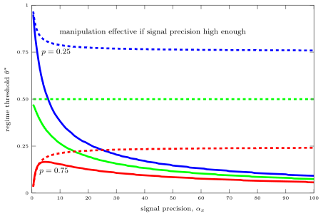
Shows the regime threshold \(\theta^*\) as functions of \(\alpha_x\). Solid lines show the regime thresholds when there is information manipulation, dashed lines show the thresholds when there is no information manipulation. If primitives are relatively favorable to the regime (say \(p=0.75\)), the coordination effect identified by Metz (2002) and the information manipulation effect pull in opposite directions, giving rise to a “hump-shaped” function. If primitives are unfavorable to the regime (say \(p=0.25\)), both forces drive \(\theta^*\) down.
Thus informative priors do not undo the central message of the benchmark model. For high \(\alpha_x\) signal-jamming is effective, \(\theta^*<\theta_{\text{MS}}^*=1-p\). High signal precision may increase the regime’s ex ante survival probability. But perhaps this is not the most interesting comparative static. What if the precision of the public signal increases? Then we run into the problem of multiplicity. For given \(\alpha _{x}\), the inequality \(\alpha _{z}/\sqrt{\alpha _{x}}<\sqrt{2\pi }\) will eventually be violated and there are multiple monotone equilibria. In this case, we lose the ability to draw sharp conclusions. What if both the precisions of the public and private information increase together? Then if the bound on the relative precision of the public information is satisfied the analysis goes through essentially as above. At a given level of the relative precision \(\alpha _{z}/\sqrt{\alpha _{x}}\), the threshold may be increasing or decreasing (depending on the relative strengths of the coordination effect and the information manipulation effect), but as the ratio \(\alpha _{z}/\sqrt{\alpha _{x}}\) becomes small the hidden action effect dominates.
D.2 Heterogeneous Informative Priors
In this section I consider an alternative and perhaps more interesting way to give citizens an uncontaminated source of information. In particular, I suppose that media outlets come in two types, some that are amenable to the regime’s message and others who resolutely report the truth. Specifically, let citizens have \(n_x\) reports from media outlets that contain the regime’s action and \(n_z\) reports from media outlets that do not contain the regime’s action. Citizens observe each of these reports with idiosyncratic noise that is jointly IID normal across them and across all media outlets with mean zero and precision \(\hat{\alpha}\). Then the information of a citizen can be represented by two representative signals \[\tag{109} x_i = \theta + a + \varepsilon_{x,i},\qquad \text{and} \qquad z_i = \theta + \varepsilon_{z,i}\] where the noise terms \(\varepsilon_{x,i}\) and \(\varepsilon_{z,i}\) are independent, jointly normally distributed, both with mean zero and precisions \(\alpha_x:=n_x \hat{\alpha}\) and \(\alpha_z:=n_z\hat{\alpha}\) respectively. This gives citizens a clean source of information \(z_i\) not affected by the regime’s manipulation. This is equivalent to giving citizens heterogeneous informative priors. It is also equivalent to giving citizens noisy signals of the hidden action \(a\) itself. Subtracting \(z_i\) from \(x_i\) gives \[ (x_i - z_i) = a + (\varepsilon_{x,i}-\varepsilon_{z,i})\] This is an unbiased signal of the regime’s action \(a\).
I consider a monotone equilibrium where the regime is overthrown for \(\theta<\theta^*\) and citizens attack, \(s(x_i,z_i)=1\), if their signals satisfy \(x_i<x^*(z_i)\). Here \(\theta^*\) is a single threshold and \(x^*:\mathbb{R}\rightarrow\mathbb{R}\) is a threshold function, both to be determined endogenously. In this case, the aggregate attack facing a regime that takes action \(a\) is \[ S(\theta,a) = \int_{-\infty}^{\infty} \Phi (\sqrt{\alpha_x}(x^*(z_i)-\theta-a))\sqrt{\alpha_z}\phi(\sqrt{\alpha_z}(z_i-\theta)) \, dz_i\] In general a citizen makes use of both types of information even though one is contaminated by \(a\) while the other is not. This is because, even considering the presence of manipulation, the \(x_i\) signals may still be more informative about \(\theta\) than the \(z_i\) signals if the precision \(\alpha_x\) is sufficiently high relative to \(\alpha_z\). Indeed, if \(\alpha_z\rightarrow0\), then we are back to the main model with only contaminated information since any uncontaminated information is too inherently noisy to be usable. Alternatively, as \(\alpha_z\) increases, the \(z_i\) signals will be given more weight, and, as \(\alpha_z\) becomes sufficiently large, the model reduces to the Morris-Shin benchmark where the only source of information is clean. For intermediate values of \(\alpha_x\) and \(\alpha_z\), matters are more complex. And, unfortunately, it is not possible to give a simple analytic characterization of the equilibrium for general signal precisions. In Figure 7, I show several numerical examples.
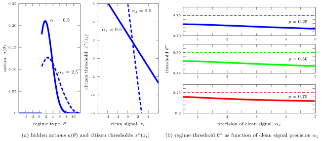
Panel (a) shows that as the precision \(\alpha_z\) of the clean signal information increases, regimes near \(\theta^*\) take smaller actions \(a(\theta)\) but \(\theta^*\) hardly changes. Citizens give more weight to their clean signal so \(x^{*}(z_i)\) is steeper, for low values of the clean signal \(z_i\) it takes a higher value of the manipulated signal \(x_i\) to induce participation in the attack. In this example the opportunity cost of participating is \(p=.25\). Panel (b) shows the regime threshold \(\theta^*\) as a function of the precision of the clean signal \(\alpha_z\). The regime still benefits from information manipulation in that \(\theta^*<\theta_{\text{MS}}^* = 1-p\). In all of these calculations, the manipulated signal has precision \(\alpha_x=.5\) and the cost function is \(C(a)=a^2/2\).
The left panel shows the equilibrium hidden actions \(a(\theta)\) and the citizen threshold function \(x^*(z_i)\) for two cases, (i) with \(\alpha_x=\alpha_z=.5\), so that the number of media outlets is the same for both kinds, and (ii) with \(\alpha_x=.5\) but \(\alpha_z=2.5\), so that there are five times as many clean sources of information. In both cases the overall level of precision is relatively low, so even though the \(x_i\) signals are manipulated while the \(z_i\) signals are clean, citizens still draw on both kinds of information. The citizen threshold function \(x^*(z_i)\) is decreasing in \(z_i\) because if a citizen gets a low \(z_i\) it takes a high \(x_i\) to induce participation in an attack. And as \(\alpha_z\) increases, the citizen threshold function \(x^*(z_i)\) becomes steeper so that the \(z_i\) are weighed more heavily and it takes an even bigger \(x_i\) to compensate for a low \(z_i\). The right panel shows the regime threshold \(\theta^*\) as a function of the clean precision \(\alpha_z\) for various opportunity costs \(p\) and for fixed \(\alpha_x=.5\) for the precision of the manipulated signal. In these examples, the \(\theta^*\) are lower than the Morris-Shin benchmarks \(1-p\) and information manipulation is effective. Moreover, in this range the thresholds are decreasing in the precision \(\alpha_z\) of the clean signal implying that, for these parameters, even an increase in the quantity of clean information increases the regime’s chances of surviving.
These examples are only suggestive of what can happen in equilibrium. Still, it is clear that introducing clean information unaffected by the regime’s manipulation does not by itself overturn the possibility that more information may increase the regime’s chances of surviving.
D.3 Manipulating Aggregate Information
To this point, information manipulation has entered through individual signals \(x_i=\theta+a+\varepsilon_i\). But the competing roles of idiosyncratic and aggregate information is generally an important determinant of equilibrium outcomes in global games. In this appendix, I show that qualitatively similar results to those obtained for the main model can be obtained if information manipulation takes place through an aggregate signal. I contrast two setups, both with idiosyncratic and aggregate information but which differ in the channel by which manipulation enters.
In the first setup, manipulation enters through the idiosyncratic information. That is, citizens have \(x_i=\theta+a+\varepsilon_{x,i}\) as usual, but also have a common or aggregate signal \(z=\theta+\varepsilon_{z}\) that is free from manipulation. Here \(\varepsilon_{x,i}\) and \(\varepsilon_z\) are jointly normally distributed, both with mean zero and precisions \(\alpha_x\) and \(\alpha_z\) respectively. This provides an appropriate benchmark against which to judge the effects of manipulation that enters through aggregate information. The second setup has \(x_i=\theta+\varepsilon_{x,i}\) but now the regime’s manipulation enters the common signal \(z=\theta+a+\varepsilon_{z}\).
Aggregate uncertainty. In both cases, I assume that the common signal \(z\) is realized after the regime chooses its action \(a(\theta)\). Thus the regime faces aggregate uncertainty and can no longer perfectly anticipate play along the equilibrium path. I consider a monotone equilibrium where the regime is overthrown ex post for \(\theta<\theta^*(z)\) and citizens attack, \(s(x_i,z)=1\), if their signals satisfy \(x_i<x^*(z)\). Here \(\theta^*:\mathbb{R}\rightarrow[0,1]\) and \(x^*:\mathbb{R}\rightarrow\mathbb{R}\) are threshold functions to be determined.
Manipulation through individual signal. In this case, the ex post aggregate attack facing a regime that takes action \(a\) is \[ S(\theta,a,z) = \Phi (\sqrt{\alpha_x}(x^*(z)-\theta-a))\] and the regime ex ante chooses \(a(\theta)\) to maximize its expected payoff, namely \[ a(\theta)\in\operatornamewithlimits{argmax}_{a\geq 0} \left[-C(a) + \int_{-\infty}^{\infty}\max[0,\theta-S(\theta,a,z)]\sqrt{\alpha_z}\phi(\sqrt{\alpha_z}(z-\theta))\,dz \right]\] The thresholds \(\theta^*(z)\) and \(x^*(z)\) are implicitly determined by indifference conditions for the regime and the citizens where the aggregate attack is \(S(\theta,a,z)\) as above and where citizens’ posterior densities are proportional to \(\phi (\sqrt{\alpha_x}(x_i-\theta-a(\theta)))\phi(\sqrt{\alpha_z}(z-\theta))\).
Manipulation through aggregate signal. In this case, the ex post aggregate attack facing a regime is \[ S(\theta,z) = \Phi (\sqrt{\alpha_x}(x^*(z)-\theta))\] independent of the regime’s hidden action \(a\). Now the regime ex ante chooses \(a(\theta)\) to maximize \[ a(\theta)\in\operatornamewithlimits{argmax}_{a\geq 0} \left[-C(a) + \int_{-\infty}^{\infty}\max[0,\theta-S(\theta,z)]\sqrt{\alpha_z}\phi(\sqrt{\alpha_z}(z-\theta-a))\,dz \right]\] And again, the thresholds \(\theta^*(z)\) and \(x^*(z)\) are implicitly determined by indifference conditions for the regime and the citizens where the aggregate attack is \(S(\theta,z)\) as above and where citizens’ posterior densities are now proportional to \(\phi (\sqrt{\alpha_x}(x_i-\theta))\phi(\sqrt{\alpha_z}(z-\theta-a(\theta)))\).
Numerical results. I solve these two models numerically.17 Several examples are shown in Figure 8. The left panel shows the hidden action function \(a(\theta)\) for the two models, each for two levels of signal precision, \(\alpha_x=.5\) and three times higher at \(\alpha_x=1.5\). Notice that, because of the aggregate uncertainty, all regimes with \(\theta>0\) take hidden actions \(a(\theta)>0\). Even with aggregate uncertainty, regimes with \(\theta<0\) know they will be overthrown.
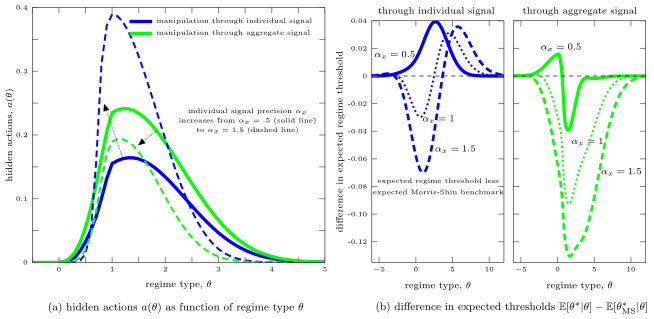
Panel (a) shows the regime’s hidden actions \(a(\theta)\) taken to maximize its expected payoff. Since there is aggregate uncertainty, for all \(\theta>0\) regimes take positive actions. The darker lines show the case of manipulation through individual signals, the lighter lines show the case of manipulation through the aggregate signal. The solid lines show low signal precisions \(\alpha_x=.5\) while the dashed lines show high signal precisions \(\alpha_x=1.5\). Panel (b) shows the difference between the average regime threshold and its Morris-Shin counterpart for the same specifications. For higher \(\alpha_x\), the average threshold tends to be lower than its Morris-Shin counterpart and the regime’s gain is relatively larger when the manipulation takes place through aggregate information. In all these examples, \(p=.25, \alpha_z=.5\) and the cost function is \(C(a)=a^2/2\).
In these examples, the extent of manipulation is typically larger when the signal precision is at the higher level \(\alpha_x = 1.5\) in the model where manipulation enters through the individual signal channel \(x_i\). But the extent of manipulation is typically smaller when the signal precision is higher if the manipulation enters through the aggregate signal channel. In both cases, the ex post regime survival outcome depends on the realization of the aggregate signal \(z\). The right panel shows the average regime threshold less the average regime threshold that would obtain in the absence of any manipulation (the corresponding Morris-Shin model with aggregate uncertainty) for each of the specifications. Here we see that for higher levels of signal precision, the average regime threshold tends to be lower than its Morris-Shin counterpart so that regimes expect to be better off. In this sense, the results are qualitatively similar to those obtained for the main model without aggregate uncertainty. This specification of the model has the additional implication that the extent of the regime’s expected gain is relatively larger if manipulation takes place through the aggregate information.
D.4 Correlation vs. Precision
In the main model a single parameter, \(\alpha\), determines both the precision of signals and, implicitly, the correlation of signals across citizens. To see this, suppose citizens have signals \[ x_i = y + \varepsilon_i\] where the noise is independent of \(y\) and is IID with mean zero and precision \(\alpha\) in the population of citizens. In order to make statements about the unconditional distribution of signals, I need to fix a prior.18 For the purposes of this appendix, there is no loss of generality in setting the prior mean to zero. I set the prior precision to \(\alpha_0>0\). Then the unconditional correlation of any pair of signals \(x_i\) and \(x_j\) is \[ \text{Corr}[x_i,x_j] = \frac{\text{Cov}[x_i,x_j]}{\text{Var}[x_i]} = \frac{\text{Var}[y]}{\text{Var}[y]+\text{Var}[\varepsilon_i]} = \frac{\alpha}{\alpha+\alpha_0}\] Thus as \(\alpha\rightarrow\infty\), the correlation \(\rightarrow 1\) for any prior precision \(\alpha_0>0\). This raises the question of whether the fall in the regime threshold \(\theta^*\) as \(\alpha\rightarrow\infty\) is driven by the increase in signal precision per se or by the implied increase in correlation.
Separating correlation from precision. To address this issue, I solve a version of the model where the signal precision can be held fixed while the signal correlation is varied. Specifically, I suppose citizens have signals \[ x_i = y + \xi_i\] where the noise \(\xi_i\) has both a common and an idiosyncratic component \[\tag{110} \xi_i = \sqrt{\rho}z +\sqrt{1-\rho}\varepsilon_i,\qquad 0<\rho<1\] The common component \(z\) is normal with mean zero and precision \(\alpha>0\) while the idiosyncratic component \(\varepsilon_i\) is independent of \(z\) and IID across citizens also with mean zero and the same precision \(\alpha\). As the correlation coefficient \(\rho\) approaches zero, this reduces to the main model of the text with uncorrelated noise \(\xi_i=\varepsilon_i\), and hence signals \(x_i=y+\varepsilon_i\). As \(\rho\) approaches one, the noise is perfectly correlated across citizens \(\xi_i=z\), and hence signals are \(x_i=y+z\) for all \(i\). This corresponds to the model with perfect coordination, as in Appendix B of the main text.
For intermediate levels of \(\rho\), the correlation of any pair of signals \(x_i\) and \(x_j\) is \[ \text{Corr}[x_i,x_j] = \frac{\text{Var}[y]+\rho\text{Var}[z]}{\text{Var}[y]+\text{Var}[\xi_i]}\] The precision of the signal noise is \[ \text{Var}[\xi_i] = \rho \text{Var}[z] + (1-\rho)\text{Var}[\varepsilon_i] = \frac{1}{\alpha}\] If we allowed the common and idiosyncratic components to have different precisions then any change in \(\rho\) would change the precision of the overall signal noise \(\xi_i\) so that we would be back to conflating the two issues. Given \(\text{Var}[\xi_i]=\text{Var}[z]=1/\alpha\), the correlation simplifies to \[\tag{111} \text{Corr}[x_i,x_j] = \frac{\alpha+\rho\alpha_0}{\alpha+\alpha_0}\] Again, as \(\alpha\rightarrow\infty\) we will have the the correlation \(\rightarrow 1\) for any prior precision \(\alpha_0>0\). Highly precise information will always be correlated across citizens, but now we can fix a particular signal precision \(\alpha\) and ask what happens as the correlation coefficient \(\rho\) changes.
Monotone equilibrium with latent correlation. Suppose the signal mean is \(y=\theta+a\) so that citizens have signals \(x_i=\theta+a+\xi_i\) where \(\xi_i\) is given by (110) above. Since the regime does not know which value of the common component \(z\) will realize, this version of the model has aggregate uncertainty. In the limit as the correlation coefficient \(\rho\rightarrow0\) this aggregate uncertainty disappears and we return to the main model.
I consider a monotone equilibrium where the regime is overthrown ex post for \(\theta<\theta^*(z)\) and citizens attack, \(s(x_i)=1\), if their signals satisfy \(x_i<x^*\). Here \(x^*\in\mathbb{R}\) is a single threshold and \(\theta^*:\mathbb{R}\rightarrow[0,1]\) is a threshold function, both to be determined endogenously.
Regime problem. In this case, the density of citizen signals \(x_i\) conditional on the signal mean \(y=\theta+a\) and on the common shock \(z\) is \[ f(x_i\,|\,y,z) := \sqrt{\frac{\alpha}{1-\rho}}\phi\left(\sqrt{\frac{\alpha}{1-\rho}}\left(x_i-y-\sqrt{\rho}z\right)\right)\] where \(\phi(\cdot)\) is the standard normal PDF. Thus, in a monotone equilibrium, if the realized common shock is \(z\) then ex post the aggregate attack facing a regime of type \(\theta\) that takes action \(a\) is \[ S(\theta,a,z) := \int_{-\infty}^{\infty} s(x_i)f(x_i\,|\,\theta+a,z)\,dx_i = \Phi\left(\sqrt{\frac{\alpha}{1-\rho}}\left(x^*-\theta-a-\sqrt{\rho}z\right)\right)\] where \(\Phi(\cdot)\) is the standard normal CDF. A high realization of the common shock \(z\) will cause citizens to observe high values of \(x_i\) and this will reduce the size of the aggregate attack. The sensitivity to \(z\) depends on the correlation coefficient \(\rho\) and is larger the more correlation there is.
Ex ante the regime chooses \(a(\theta)\) to maximize its expected payoff, namely \[\tag{112} a(\theta)\in\operatornamewithlimits{argmax}_{a\geq 0} \left[-C(a) + \int_{-\infty}^{\infty}\max[0,\theta-S(\theta,a,z)]\sqrt{\alpha}\phi(\sqrt{\alpha}z)\,dz \right]\] Ex post the regime’s threshold \(\theta^*(z)\) is determined by the indifference condition \[\tag{113} \theta^*(z) = S(\theta^*(z),a(\theta^*(z)),z) + C(a(\theta^*(z))),\qquad \text{for each $z\in\mathbb{R}$}\] Both \(a(\theta)\) and \(\theta^*(z)\) implicitly depend on the citizen threshold \(x^*\).
Citizen problem. Conditional on \(\theta\), the signals \(x_i\) are normally distributed with mean \(y(\theta)=\theta+a(\theta)\) and precision \(\alpha\). Thus the citizens’ posterior for \(\theta\) is \[ \pi (\theta\,|\,x_i) = \frac{\sqrt{\alpha}\phi(\sqrt{\alpha}(x_i-y(\theta)))}{\int_{-\infty}^{\infty}\sqrt{\alpha}\phi(\sqrt{\alpha}(x_i-y(\theta)))\,d\theta}\] A citizen attacks, \(s(x_i)=1\), if and only if the probability of the regime being overthrown is at least \(p\). If the common shock \(z\) was known, the posterior probability of the regime being overthrown would be \[ \int_{-\infty}^{\theta^*(z)}\pi(\theta\,|\,x_i)\, d\theta\] but, because \(z\) is not known, citizens also have to integrate with respect to the density of \(z\) so that the indifference condition characterizing the citizen threshold \(x^*\) is \[\tag{114} \int_{-\infty}^{\infty}\int_{-\infty}^{\theta^*(z)}\pi(\theta\,|\,x^*)\,d\theta \sqrt{\alpha}\phi(\sqrt{\alpha}z)\,dz = p\] The correlation coefficient \(\rho\) matters for individual citizens’ decisions through the hidden actions \(a(\theta)\) and the regime thresholds \(\theta^*(z)\), not in any direct fashion.
Numerical examples. I compute numerical solutions for this model with correlation by solving equations (112), (113) and (114) simultaneously for the functions \(a(\theta)\) and \(\theta^* (z)\) and the scalar \(x^*\). Figure 9 shows the ex ante expected regime threshold as a function of the correlation coefficient \(\rho\) for three different levels of the signal precision.
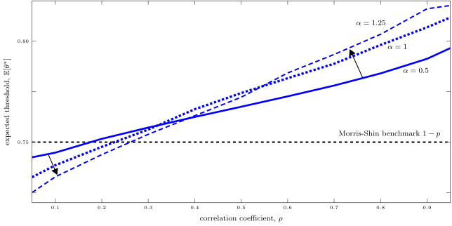
The expected regime threshold \(\mathbb{E}[\theta^*]\) as a function of the correlation coefficient \(\rho\) for various levels of the signal precision \(\alpha\). For fixed \(\alpha\), the expected regime threshold is increasing in \(\rho\), suggesting that increasing correlation works against the regime (it is more likely to be overthrown). At low levels of \(\rho\), an increase in \(\alpha\) reduces the expected regime threshold, as in the main model. At high levels of \(\rho\), an increase in \(\alpha\) increases the expected regime threshold, as in the perfect coordination model in Appendix B in the main text. In all these examples, \(p=.25\) and the cost function is \(C(a)=a^2/2\).
In these examples the individual opportunity cost is \(p=.25\) so that the Morris-Shin benchmark is \(\theta^*_{\text{MS}}=1-p=.75\). As \(\rho\rightarrow0\) we have the main model with information manipulation and with correlation in signals only because of increasing precision. For these parameters the equilibrium threshold \(\theta^*\) (which is deterministic when \(\rho=0\), since then there is no aggregate uncertainty) is less than the Morris-Shin benchmark and is decreasing in the signal precision \(\alpha\). Given that \(p<.50\), this is exactly what we expect from Proposition 3 in the main text.
Now fix a particular level of \(\alpha\). As the correlation coefficient \(\rho\) increases we have that the expected regime threshold rises. More underlying latent correlation for a given level of signal precision means that the regime expects to be worse off in the sense that it is more likely to be overthrown. As \(\rho\) increases the expected regime threshold is driven above the Morris-Shin benchmark \(1-p\) for a fixed level of \(\alpha\). The total correlation in signals depends on both the latent correlation in the noise governed by \(\rho\) and on the level of signal precision \(\alpha\). As \(\alpha\) increases, the total correlation increases for any level of \(\rho\), as in equation (111). Here we see that, for high levels of \(\rho\), an increase in signal precision \(\alpha\) continues to shift the expected regime threshold even higher.
These examples also agree with the analytic results in Appendix B in the main text where the regime is confronted by a single perfectly coordinated agent (i.e., \(\rho=1\)) for some arbitrary level of signal precision \(\alpha\). In that perfect correlation case, as the signal precision becomes arbitrarily high, \(\alpha\rightarrow\infty\), the regime threshold \(\theta^*\rightarrow1\) so that all the fragile regimes \(\theta\in[0,1)\) are overthrown. This is the exact opposite of the result with uncorrelated signals (i.e., \(\rho=0\)) where \(\alpha\rightarrow\infty\) implies the regime threshold \(\theta^*\rightarrow0\) so that all the fragile regimes \(\theta\in[0,1)\) survive. Overall, this suggests that it is the increase in signal precision rather than the implied increase in total correlation that is responsible for the regime threshold being driven to zero in the main model. Correlation per se is not in a regime’s interest. At any given level of signal precision, the regime would prefer it if its opponents were less coordinated.
See Carlsson and Damme (1993) and Morris and Shin (1998, 2003). Other political economy applications of global games include Boix and Svolik (2013), Bueno de Mesquita (2010), Chassang (2010) and Shadmehr and Bernhardt (2011).↩︎
The supplementary appendix provides simple micro-foundations for this form of media report and also considers heterogeneous media outlets, some of which pass on the manipulation and some of which do not.↩︎
I thank an anonymous referee for suggesting this line of argument. Observe also that since the regime’s payoff \(B(\theta,S)-C(a)\) is separable in \(a\), the condition \(B_{\theta S}\leq 0\) implies that the regime’s indifference curves in \((S,a)\) satisfy a standard single-crossing property.↩︎
This first order condition may have zero or two solutions. If there are two solutions, it is straightforward to show that only the larger of these satisfies the second order condition.↩︎
Perhaps surprisingly, this result does not depend on a diffuse prior for \(\theta\). The supplementary appendix shows how this limiting result still obtains even in the case of informative priors.↩︎
In my model the “message” \(y(\theta)\) is observed with noise. See Blume et al. (2007) for a Crawford and Sobel (1982) model where information receivers sometimes see only noise rather than the sender’s intended message. Blume et al. (2007) show that the presence of noise generally allows for more communication than the noiseless benchmark and that for low levels of noise this can be welfare-improving.↩︎
Chase and Mulvenon (2002), by contrast, emphasize the Chinese regime’s use of more traditional authoritarian methods in cracking down on online dissent. Kalathil and Boas (2003) also discuss related efforts by autocratic regimes to counteract the internet in Cuba, Saudi Arabia, and elsewhere. Soley (1987) discusses earlier efforts by the Cuban regime to counteract US-based satellite radio and television broadcasts.↩︎
I thank an anonymous referee for suggesting this proof.↩︎
In an industrial organization context, however, see Bose et al. (2006) for an information cascade problem where an informed monopolist seeks to control the ensuing herd behavior of consumers.↩︎
See Baliga and Sjöström (2012) for a related model with cheap talk instead of costly signaling.↩︎
Following Mullainathan and Shleifer (2005), this can be interpreted as follows: the marginal cost of producing information is zero and Bertrand competition between symmetric media outlets has driven the price of information to zero. To be consistent with this interpretation, the number of symmetric media outlets should be \(n\geq2\).↩︎
If different media outlets had different preferences for accommodating the regime, then citizens would not weigh them equally. An extension involving heterogeneous media outlets is given in Appendix D.2 below.↩︎
In Mullainathan and Shleifer (2005), if individuals have heterogeneous preferences — say some preferring slant one way, some the other — then competitive media outlets differentiate and the market for information is segmented in a manner that serves to align individuals’ preference for biased information with the reports they actually receive. By contrast, in Gentzkow and Shapiro (2006) market competition serves to reduce the amount of bias.↩︎
The use of a coordination game to model regime change is common in the political economy literature — see for example Kuran (1989, 1995) or more recently Fearon (2006) and Bueno de Mesquita (2010).↩︎
Of these, Lohmann (1993) is most closely related to this paper. In that model, there is a large agent that takes a political action in response to the collective decisions of many small voters, but in her setting the large agent has preferences that align with the median voter whereas the large agent in this model, the regime, is diametrically opposed to the preferences of the citizens.↩︎
In a binary action game like the one in this paper, individual citizens who do not attack implicitly collaborate with the regime in that they make it harder to raise an aggregate \(S\) large enough to force regime change.↩︎
These calculations keep the precision \(\alpha_z\) of aggregate information fixed and sufficiently low relative to the precision of idiosyncratic information that there is no multiplicity of monotone equilibria.↩︎
In the model I assumed an improper uniform prior on \(\mathbb{R}\) for which the unconditional correlation is not defined.↩︎