---
abstract: |
We study the procompetitive gains from international trade in a quantitative model with endogenously variable markups. We find that trade can significantly reduce markup distortions if two conditions are satisfied: (i) there is extensive misallocation and (ii) opening to trade exposes hitherto dominant producers to greater competitive pressure. We measure the extent to which these two conditions are satisfied in Taiwanese producer-level data. Versions of our model consistent with the Taiwanese data predict that opening up to trade strongly increases competition and reduces markup distortions by up to one-half, thus significantly reducing productivity losses due to misallocation.
*JEL classifications*: F11, F12, L11, L13, O47.
appendix-pdf-url: "https://chrisedmond.net/Edmond%20Midrigan%20Xu%20Appendix%20March%202015.pdf"
author:
- Chris Edmond, Virgiliu Midrigan, and Daniel Yi Xu
bibliography:
- ../gains-from-trade-ref.bib
build-date: 2026-09-17
csl: csl/chicago-author-date.csl
date: October 2015
doi: 10.1257/aer.20120549
link-citations: true
math-overflow: linebreak
mathjax-url: "https://cdn.jsdelivr.net/npm/mathjax@4/tex-chtml.js"
pdf-url: "https://chrisedmond.net/Edmond%20Midrigan%20Xu%20AER%202015.pdf"
published-in: American Economic Review
replication-url: "https://chrisedmond.net/EMX%20replication%20materials.zip"
title: Competition, Markups, and the Gains from International Trade
version: v1
---
*Acknowledgments:* We thank four anonymous referees for valuable comments and suggestions. We have also benefited from discussions with Fernando Alvarez, Costas Arkolakis, Andrew Atkeson, Ariel Burstein, Vasco Carvalho, Andrew Cassey, Arnaud Costinot, Jan De Loecker, Dave Donaldson, Ana Cecilia Fieler, Oleg Itskhoki, Phil McCalman, Markus Poschke, Andrés Rodríguez-Clare, Barbara Spencer, Iván Werning, and from numerous conference and seminar participants. We also thank Andres Blanco, Sonia Gilbukh, Jiwoon Kim and Fernando Leibovici for their excellent research assistance. We thank the National Science Foundation for financial support under grant SES-1156168. Edmond also thanks the Australian Research Council for financial support under grant DP-150101857. Midrigan also thanks the Alfred P. Sloan foundation for financial support. The authors declare that they have no relevant or material financial interests that relate to the research described in this paper. Midrigan is a consultant at the Federal Reserve Bank of Minneapolis.
*Affiliations:* Chris Edmond, University of Melbourne. Virgiliu Midrigan, New York University and NBER. Daniel Yi Xu, Duke University and NBER.
# 1 Introduction
Can international trade significantly reduce product market distortions? We study this question in a quantitative trade model with endogenously variable markups. In such a model, markup dispersion implies that resources are *misallocated* and that aggregate productivity is low. By exposing producers to greater competition, international trade may reduce markup dispersion thereby reducing misallocation and increasing aggregate productivity. Our goal is to use producer-level data to quantify these *procompetitive effects*.
We study these procompetitive effects in the model of Atkeson and Burstein ([2008](#ref-ATKE/BURS/08)). In this model, any given sector has a small number of producers who engage in *oligopolistic competition*. The demand elasticity for any given producer is decreasing in its market share and hence its markup is increasing in its market share. By reducing the market shares of dominant producers, international trade can reduce markups and markup dispersion. The Atkeson and Burstein ([2008](#ref-ATKE/BURS/08)) model is particularly useful for us because it implies a *linear* relationship between (inverse) producer-level markups and market shares, which in turn makes the model straightforward to parameterize.
We find that trade can significantly reduce markup distortions if two conditions are satisfied: (i) there is extensive misallocation, and (ii) international trade does in fact put producers under greater competitive pressure. The first condition is obvious --- if there is no misallocation, there is no misallocation to reduce. The second condition is more subtle. Trade has to increase the degree of effective competition prevailing amongst producers within a market. If both domestic and foreign producers have similar productivities within a given sector, then opening to trade exposes them to genuine *head-to-head competition* that reduces market power thereby reducing markups and markup dispersion. By contrast, if there are large cross-country differences in productivity within a given sector, then opening to trade may allow producers from one country to substantially increase their market share in the other country, thereby increasing markups and markup dispersion so that the procompetitive 'gains' from trade are negative.
We quantify the model using 7-digit Taiwanese manufacturing data. We use this data to discipline two key determinants of the extent of misallocation: (i) the elasticity of substitution across sectors, and (ii) the equilibrium distribution of producer market shares. The elasticity of substitution across sectors plays a key role because it determines the extent to which producers facing little competition in their own sector can raise markups. We pin down this elasticity by requiring that our model fits the cross-sectional relationship between measures of markups and market shares that we observe in the Taiwanese data. We pin down the parameters of the producer-level productivity distribution and fixed costs of operating and exporting by requiring that the model reproduces key moments of the distribution of market shares within and across sectors in the Taiwanese data.
The Taiwanese data feature a large amount of both dispersion and concentration in producer-level market shares and a strong relationship between market shares and measured markups. Interpreted through the lens of the model, this implies a significant amount of misallocation and hence the possibility of significant productivity gains from reduced markup distortions.
Given this misallocation, the model predicts large procompetitive gains if, within a given sector, domestic producers and foreign producers have relatively similar levels of productivity so that more trade increases the degree of competition prevailing among producers. This feature of the model is largely determined by the *cross-country correlation* in sectoral productivity. We choose the amount of correlation in sectoral productivity so that the model reproduces standard estimates of the elasticity of trade flows with respect to changes in variable trade costs. As the amount of correlation increases, there is less cross-country variation in producers' productivity. Consequently, small changes in trade costs have relatively larger effects on trade flows --- in short, the *trade elasticity* is increasing in the amount of cross-country correlation. To match standard estimates of the trade elasticity, the benchmark model requires a relatively high 0.94 cross-country correlation in sectoral draws. This high correlation also allows the model to reproduce the strong positive relationship between a sector's share of domestic sales and its share of imports that we observe in the data --- i.e., reproduces the fact that sectors with relatively large, productive firms are also sectors with relatively large import shares.
Given this high degree of correlation, opening to trade indeed reduces markup dispersion and increases aggregate productivity. For the benchmark model, calibrated to Taiwan's import share, opening to trade reduces markup distortions by about one-fifth and increases aggregate productivity by 12.4 percent relative to autarky. In short we find that, yes, opening to trade can lead to a quantitatively significant reduction in misallocation. We also find that these procompetitive effects are strongest near autarky --- the procompetitive effects are more important for an economy opening from autarky to a 10 percent import share than for an economy increasing its openness from a 10 to 20 percent import share.
In the model, a given producer's productivity has both a sector-specific component and an idiosyncratic component, both drawn from Pareto distributions. In our benchmark model, the sectoral draws are correlated across countries while the idiosyncratic draws are not. We consider an extension of the model in which the idiosyncratic draws are also correlated across producers in a given sector in different countries. This extension is motivated by the observation that sectors with high concentration amongst domestic producers are also sectors with high import penetration. While our benchmark model cannot reproduce this feature of the data, our extension with correlated idiosyncratic draws can. This extension predicts an even larger role for trade in reducing markup distortions because countries import more of exactly those goods for which the domestic market is more distorted. In this version of the model, trade eliminates about one-third of the productivity losses from misallocation.
We consider a number of robustness checks on our benchmark model --- including allowing for heterogeneity in sector-level tariffs, introducing labor market distortions, and changing the mode of competition from Cournot to Bertrand, amongst others. Our main findings are robust to these alternative specifications. We also study an extension of the model in which we introduce capital and elastic labor supply and show that the procompetitive gains from trade are even larger. Finally, we study a version of the model with free-entry and show that versions of the free-entry model that reproduce the salient features of the Taiwanese data continue to predict significant procompetitive gains from trade.
**Markups, misallocation, and trade.** Recent papers by Restuccia and Rogerson ([2008](#ref-REST/ROGE/08)), Hsieh and Klenow ([2009](#ref-HSIE/KLEN/09)) and others show that misallocation of factors of production can substantially reduce aggregate productivity. We focus on the role of markup variation as a source of misallocation.[^1] We find that, by reducing markup dispersion, trade can play a powerful role in reducing misallocation and can thereby increase aggregate productivity.
The possibility that opening an economy to trade may lead to welfare gains from increased competition is, of course, one of the oldest ideas in economics. But standard quantitative trade models, such as the perfect competition model of Eaton and Kortum ([2002](#ref-EATO/KORT/02)) or the monopolistic competition models with constant markups of Melitz ([2003](#ref-MELI/03)) and Chaney ([2008](#ref-CHAN/08)), cannot capture this procompetitive intuition.
Perhaps more surprisingly, existing trade models that *do* feature variable markups do not generally predict procompetitive gains. For example, the Bernard et al. ([2003](#ref-BERN/ETAL/03), hereafter BEJK) model of Bertrand competition results in an endogenous distribution of markups, that, due to specific functional form assumptions, is *invariant* to changes in trade costs and has exactly *zero* procompetitive gains.[^2] Similarly, in the monopolistic competition models with non-CES demand[^3] studied by Arkolakis et al. ([2012a](#ref-ACDR/12), hereafter ACDR), the markup distribution is likewise invariant to changes in trade costs and there are in fact *negative* procompetitive 'gains' from trade.
The reason models with variable markups yield conflicting predictions regarding the procompetitive gains from trade is that, as emphasized by ACDR, what really matters for these effects is the *joint distribution* of markups and employment. The response of this joint distribution to a reduction in trade costs depends on the parameterization of the model, and in particular the amount of cross-country correlation in productivity draws. We show that versions of our model with low correlation do indeed predict negative procompetitive gains. But such parameterizations also imply both (i) low aggregate trade elasticities, and (ii) a weak or negative relationship between a sector's share of domestic sales and its share of imports --- and thus are inconsistent with empirical evidence.
**Empirical literature on markups and trade.** There is a large empirical literature on producer markups and trade. Important early examples include Levinsohn ([1993](#ref-LEVI/93)), Harrison ([1994](#ref-HARR/94)), and Krishna and Mitra ([1998](#ref-KRIS/MITR/98)). Tybout ([2003](#ref-TYBO/01)) reviews this literature and concludes that "in *every* country studied, relatively high sector-wide exposure to foreign competition is associated with lower price-cost margins, and the effect is concentrated in *larger* plants." More recently, Feenstra and Weinstein ([2010](#ref-FEEN/WEIN/10)) infer large markup reductions from observed changes in US market shares from 1992--2005. De Loecker et al. ([2014](#ref-DELO/ETAL/12)) study the effects of India's tariff reductions on both final goods and inputs and find that the *net* effect was in fact an *increase* in markups --- because input tariffs fell, so did the costs of final goods producers. When they condition on the effects of trade liberalization through inputs, however, De Loecker et al. ([2014](#ref-DELO/ETAL/12)) find that the markups of final goods producers fall. Their results are thus consistent with our benchmark model.
There are important conceptual differences between the effects of trade in this literature and procompetitive gains through *reduced misallocation*. Documenting changes in the domestic markup distribution following a trade liberalization does not tell us whether misallocation has gone down or not. Again, what matters for misallocation is the response of the joint distribution of employment and markups of all producers, including exporters.
**Trade flows and the gains from trade.** Our focus on the gains from trade is related to the work of Arkolakis et al. ([2012b](#ref-ARKO/ETAL/11), hereafter ACR), who show that the total gains from trade are identical in a large class of models and are summarized by the aggregate trade elasticity. Interestingly, we find that for our benchmark parameterization the ACR formula in fact provides an excellent approximation to the total gains from trade in our setup with variable markups.
That said, while the total gains from trade in our benchmark parameterization are well-approximated by the ACR formula, our model nevertheless predicts important procompetitive gains from trade. That is, opening up to trade substantially reduces markup distortions. Moreover, our model predicts that the gains from trade for two otherwise identical countries are larger for a country that has not yet reformed its product markets. Such differences in product market distortions are endogenously reflected in differences in the aggregate trade elasticity itself --- which is precisely why the ACR formula can capture these procompetitive effects. Put differently, there can be important procompetitive gains in our model even when the ACR formula works well.[^4]
The remainder of the paper proceeds as follows. [Section 2](#sec:Model) presents the model. [Section 3](#sec:Data) gives an overview of the data and [Section 4](#sec:Calibration) explains how we use that data to quantify the model. [Section 5](#sec:Gains) presents our benchmark results on the gains from trade. [Section 6](#sec:Robustness) conducts a number of robustness checks. [Section 7](#sec:Extensions) presents results for two extensions of our benchmark model, (i) trade between asymmetric countries, and (ii) free entry and an endogenous number of competitors per sector. [Section 8](#sec:Conclusions) concludes.
# 2 Model
The economy consists of two symmetric countries, Home and Foreign. In keeping with standard assumptions in the trade literature, we assume a static environment with a single factor of production, labor, that is in inelastic supply and immobile between countries. We focus on describing the Home country in detail. We indicate Foreign variables with an asterisk.
## 2.1 Final Good Producers
Perfectly competitive firms in each country produce a homogeneous final consumption good $Y$ using inputs $y(s)$ from a continuum of *sectors* $$\tag{1}
Y = \left(\int_0^1 y(s)^{\frac{\theta-1}{\theta}}\,ds \right)^{\frac{\theta}{\theta-1}}\, ,$$ where $\theta>1$ is the elasticity of substitution *across* sectors $s\in[0,1]$. Importantly, each sector consists of a *finite* number of domestic and foreign intermediate producers. In sector $s$, output is produced using $n(s)\in\mathbb{N}$ domestic and $n(s)$ imported intermediate inputs $$\tag{2}
y(s) = \left(\sum_{i=1}^{n(s)} y^{\text{H}}_i(s)^{\frac{\gamma-1}{\gamma}} + \sum_{i=1}^{n(s)} y^{\text{F}}_{i}(s)^{\frac{\gamma-1}{\gamma}} \right)^{\frac{\gamma}{\gamma-1}}\, ,$$ where $\gamma>\theta$ is the elasticity of substitution across goods $i$ *within* a particular sector $s\in[0,1]$.
In our benchmark model, the number of potential producers $n(s)$ in sector $s$ is exogenous and the same in both countries. In [Section 7](#sec:Extensions) below we consider an extension of the benchmark model with *free entry* that makes the number of producers endogenous and varying across countries.[^5]
## 2.2 Intermediate Goods Producers
Intermediate good producer $i$ in sector $s$ produces output using labor $$\tag{3}
y_i (s) = a_i (s) l_i(s)\, ,$$ where producer-level productivity $a_i(s)$ is drawn from a distribution that we discuss in detail in [Section 4](#sec:Calibration) below.
**Trade costs.** An intermediate good producer sells output to final good producers located in both countries. Let $y^{\text{H}}_i(s)$ denote the amount sold by a Home intermediate good producer to Home final good producers and similarly let $y^{\ast\text{H}}_i(s)$ denote the amount sold by a Home intermediate good producer to Foreign final good producers. The resource constraint for Home intermediate good producers is $$\tag{4} y_i(s) = y^{\text{H}}_i(s) + \tau \, y^{\ast\text{H}}_i(s)\, ,$$ where $\tau\geq1$ is an iceberg trade cost, i.e., $\tau \, y^{\ast\text{H}}_i(s)$ must be shipped for $y^{\ast\text{H}}_i(s)$ to arrive abroad. Foreign intermediate producers face symmetric trade costs. We let $y^*_i(s)$ denote their output and note that the resource constraint facing Foreign intermediate producers is $$\tag{5} y^*_i(s) = \tau\, y^{\text{F}}_i(s) + y^{\ast\text{F}}_i(s)\, ,$$ where $y^{\ast\text{F}}_i(s)$ denotes the amount sold by a Foreign intermediate good producer to Foreign final good producers and $y^{\text{F}}_i(s)$ denotes the amount sold by a Foreign intermediate good producer to Home final good producers.
**Demand for intermediate inputs.** Final good producers buy intermediate goods from Home producers at prices $p^{\text{H}}_{i}(s)$ and from Foreign producers at prices $p^{\text{F}}_i(s)$. Consumers buy the final good at price $P$. A final good producer chooses intermediate inputs $y^{\text{H}}_{i}(s)$ and $y^{\text{F}}_{i}(s)$ to maximize profits: $$\tag{6}
PY - \int_0^1 \Big(\sum_{i=1}^{n(s)} p^{\text{H}}_{i}(s) y^{\text{H}}_{i}(s) + \tau \sum_{i=1}^{n(s)} p^{\text{F}}_{i}(s) y^{\text{F}}_{i}(s)\Big)\,ds \, ,$$ subject to ([1](#eq:Y)) and ([2](#eq:y(s))). The solution to this problem gives the demand functions: $$\tag{7}
y^{\text{H}}_i(s) = \left(\frac{p^{\text{H}}_i(s)}{p(s)}\right)^{-\gamma} \, \left(\frac{p(s)}{P}\right)^{-\theta} Y\, ,$$ and $$\tag{8}
y^{\text{F}}_i(s) = \left(\frac{\tau p^{\text{F}}_i(s)}{p(s)}\right)^{-\gamma} \, \left(\frac{p(s)}{P}\right)^{-\theta} Y\, ,$$ where the aggregate and sectoral price indexes are $$\tag{9}
P = \left(\int_0^1 p(s)^{1-\theta}\,ds \right)^{\frac{1}{1-\theta}}\, ,$$ and $$\tag{10}
p(s) = \left(\sum_{i=1}^{n(s)} \phi^{\text{H}}_{i}(s) p^{\text{H}}_i(s)^{1-\gamma} + \tau^{1-\gamma}\,\sum_{i=1}^{n(s)} \phi^{\text{F}}_{i}(s) p^{\text{F}}_{i}(s)^{1-\gamma} \right)^{\frac{1}{1-\gamma}}\, ,$$ and where $\phi^{\text{H}}_{i}(s)\in\{0,1\}$ is an indicator function that equals one if a producer operates in the Home market (its domestic market) and likewise $\phi^{\text{F}}_{i}(s)\in\{0,1\}$ is an indicator function that equals one if a Foreign producer operates in the Home market (its export market).
**Market structure.** An intermediate good producer faces the demand system given by equations ([7](#eq:yHi(s)))-([10](#eq:p(s))) and engages in *Cournot competition* within its sector.[^6] That is, each individual firm chooses a quantity $y^{\text{H}}_{i}(s)$ or $y^{*\text{H}}_{i}(s)$ taking as given the quantity decisions of its competitors in sector $s$. Due to constant returns, the problem of a firm in its domestic market and its export market can be considered separately.
**Fixed costs.** There are fixed costs $f_d$ and $f_x$ of operating in the domestic and foreign market respectively. Both of these are denominated in units of domestic labor. A firm can choose to produce zero units of output for the domestic market to avoid paying the fixed cost $f_d$. Similarly, a firm can choose to produce zero units of output for the export market to avoid paying the fixed cost $f_x$. We introduce fixed operating costs in order to allow the model to match the lower tail of the distribution of firm size in the data.
**Domestic market.** Taking the wage $W$ as given, the problem of a Home firm in its domestic market can be written $$\tag{11} \pi^{\text{H}}_i(s) \, := \, \max_{y^{\text{H}}_i(s)\, , \,\phi^{\text{H}}_i(s)} \, \Big[\Big(p^{\text{H}}_{i}(s)-\frac{W}{a_i(s)}\Big)y^{\text{H}}_i(s)- Wf_d\Big]\phi^{\text{H}}_i(s) \, ,$$ subject to the demand system above. The solution to this problem is characterized by a price that is a markup over marginal cost $$\tag{12}
p^{\text{H}}_{i}(s) = \frac{\varepsilon^{\text{H}}_i(s)}{\varepsilon^{\text{H}}_i(s)-1} \, \frac{W}{a_i(s)}\, ,$$ where $\varepsilon^{\text{H}}_i(s)>1$ is the demand elasticity facing the firm in its domestic market. With the nested CES demand system above and Cournot competition, it can be shown that this demand elasticity is a weighted *harmonic* average of the underlying elasticities of substitution $\theta$ and $\gamma$, specifically $$\tag{13}
\varepsilon^{\text{H}}_i(s) = \left(\omega^{\text{H}}_i(s)\frac{1}{\theta} +(1-\omega^{\text{H}}_i(s))\frac{1}{\gamma}\right)^{-1}\, ,$$ where $\omega^{\text{H}}_i(s)\in[0,1]$ is the firm's share of sectoral revenue in its domestic market $$\tag{14} \omega^{\text{H}}_i(s) := \frac{p^{\text{H}}_{i}(s)y^{\text{H}}_{i}(s)}{\sum_{i=1}^{n(s)} p^{\text{H}}_{i}(s)y^{\text{H}}_{i}(s)+\tau \sum_{i=1}^{n(s)} p^{\text{F}}_{i}(s)y^{\text{F}}_{i}(s)} = \left(\frac{p^{\text{H}}_i(s)}{p(s)}\right)^{1-\gamma}\, .$$ For short, we refer to $\omega^{\text{H}}_i(s)$ as a Home firm's domestic *market share*.
**Export market.** The problem of a Home firm in its export market is essentially identical except that to export (operate abroad) it pays a fixed cost $f_x$ rather than $f_d$ so that its problem is $$\tag{15} \pi^{*\text{H}}_i(s) \, := \, \max_{y^{*\text{H}}_i(s)\, , \,\phi^{*\text{H}}_i(s)} \, \Big[\Big(p^{*\text{H}}_{i}(s)-\frac{W}{a_i(s)}\Big)y^{*\text{H}}_i(s)- Wf_x\Big]\phi^{*\text{H}}_i(s) \, ,$$ subject to the demand system abroad. Prices are again a markup over marginal cost $$\tag{16}
p^{*\text{H}}_{i}(s) = \frac{\varepsilon^{*\text{H}}_i(s)}{\varepsilon^{*\text{H}}_i(s)-1} \, \frac{W}{a_i(s)}\, ,$$ where $\varepsilon^{*\text{H}}_i(s)>1$ is the demand elasticity facing the firm in its export market $$\tag{17} \varepsilon^{*\text{H}}_i(s) = \left(\omega^{*\text{H}}_i(s)\frac{1}{\theta} +(1-\omega^{*\text{H}}_i(s))\frac{1}{\gamma}\right)^{-1}\, ,$$ and where $\omega^{*\text{H}}_i(s)\in[0,1]$ is the firm's share of sectoral revenue in its export market $$\tag{18} \omega^{*\text{H}}_i(s) := \frac{\tau p^{*\text{H}}_{i}(s)y^{*\text{H}}_{i}(s)}{\tau \sum_{i=1}^{n(s)} p^{*\text{H}}_{i}(s)y^{*\text{H}}_{i}(s) + \sum_{i=1}^{n(s)} p^{*\text{F}}_{i}(s)y^{*\text{F}}_{i}(s)}\, .$$ For short, we refer to $\omega^{*\text{H}}_i(s)$ as a Home firm's export market share.
**Market shares and demand elasticity.** In general, each firm faces a different, endogenously determined, demand elasticity. The demand elasticity is given by a weighted average of the within-sector elasticity $\gamma$ and the across-sector elasticity $\theta<\gamma$. Firms with a small market share within a sector (within a given country) compete mostly with other firms in their own sector and so face a relatively high demand elasticity, closer to the within-sector $\gamma$. Firms with a large market share face relatively more competition from firms in other sectors than they do from firms in their own sector and so face a relatively low demand elasticity, closer to the across-sector $\theta$. The markup a firm charges is an increasing *convex* function of its market share. An infinitesimal firm charges a markup of $\gamma/(\gamma-1)$, the smallest possible in this model. At the other extreme, a pure monopolist charges a markup of $\theta/(\theta-1)$, the largest possible in this model. Because of the convexity, a mean-preserving spread in market shares will increase the average markup.
The extent of *markup dispersion* across firms depends both on the *gap* between $\theta$ and $\gamma$ and on the extent of dispersion in market shares. In the special case where $\theta=\gamma$, the demand elasticity is constant and independent of the dispersion in market shares and the model collapses to a standard trade model with constant markups. But if $\theta$ is substantially smaller than $\gamma$, then even a modest change in market share dispersion can have a large effect on markup dispersion and hence a large effect on aggregate productivity.
Notice also that a firm operating in both countries will generally have different market shares in each country and consequently face different demand elasticities and charge different markups in each country.
**Market shares and markups.** The formula ([13](#eq:demand_elasticity)) for a firm's demand elasticity implies a linear relationship between a firm's *inverse markup* and its market share $$\tag{19}
\frac{1}{\mu_i^{\text{H}}(s)} = \frac{\gamma-1}{\gamma} - \left(\frac{1}{\theta}-\frac{1}{\gamma}\right) \omega^{\text{H}}_i(s)\, .$$ where $\mu_i^{\text{H}}(s):=\varepsilon^{\text{H}}_i(s)/(\varepsilon^{\text{H}}_i(s)-1)$ denotes the firm's gross markup from ([12](#eq:pricing)). Since $\theta<\gamma$, the coefficient on the market share $\omega^{\text{H}}_i(s)$ is negative. Within a sector $s$, firms with relatively high market shares have low demand elasticity and high markups. As discussed in [Section 4](#sec:Calibration) below, the strength of this relationship plays a key role in identifying plausible magnitudes for the gap between the elasticity parameters $\theta$ and $\gamma$.
**Operating decisions.** Each firm must pay a fixed cost $f_d$ to operate in its domestic market and a fixed cost $f_x$ to operate in its export market. A Home firm operates in its domestic market so long as $$\tag{20} \Big(p^{\text{H}}_{i}(s)-\frac{W}{a_i(s)}\Big)y^{\text{H}}_i(s)\geq Wf_d$$ Similarly, a Home firm operates in its export market so long as $$\tag{21} \Big(p^{*\text{H}}_{i}(s)-\frac{W}{a_i(s)}\Big)y^{*\text{H}}_i(s) \geq Wf_x$$ There are multiple equilibria in any given sector. Different combinations of firms may choose to operate, given that the others do not. As in Atkeson and Burstein ([2008](#ref-ATKE/BURS/08)), within each sector $s$ we place firms in the order of their physical productivity $a_i(s)$ and focus on equilibria in which firms sequentially decide on whether to operate or not: the most productive decides first (given that no other firm operates), the second most productive decides second (given that no other less productive firm operates), and so on.[^7]
## 2.3 Market Clearing
In each country there is a representative consumer that inelastically supplies one unit of labor and consumes the final good. Let $l^{\text{H}}_i(s)$ denote the labor a Home firm uses in production for its domestic market and similarly let $l^{*\text{H}}_i(s)$ denote the labor a Home firm uses in production for its export market. The labor market clearing condition is then $$\tag{22} \int_0^1 \Big(\sum_{i=1}^{n(s)} (l^{\text{H}}_i(s)+f_d)\phi^{\text{H}}_i(s) + \sum_{i=1}^{n(s)} (l^{*\text{H}}_i(s)+f_x)\phi^{*\text{H}}_i(s)\Big)\,ds = 1\, ,$$ and the market clearing condition for the final good is simply $C=Y$.
## 2.4 Aggregate Productivity and Markups
**Aggregation.** The quantity of final output in each country can be written $$\tag{23} Y = A \tilde{L},$$ where $A$ is the endogenous level of aggregate productivity and $\tilde{L}$ is the aggregate amount of labor employed *net of fixed costs*. Using the firms' optimality conditions and the market clearing condition for labor, it is straightforward to show that aggregate productivity is a *quantity-weighted* harmonic mean of firm productivities $$\tag{24}
A = \left(\int_0^1 \Big(\sum_{i=1}^{n(s)} \frac{1}{a_i (s)}\,\frac{y^{\text{H}}_i(s)}{Y} + \tau \sum_{i=1}^{n(s)} \frac{1}{a_i (s)}\,\frac{y^{*\text{H}}_i(s)}{Y} \Big)\,ds\right)^{-1}\, .$$ Now denote the aggregate (economy-wide) markup by $$\tag{25} \mu := \frac{P}{W/A}\, ,$$ that is, aggregate price divided by aggregate marginal cost. It is straightforward to show that the aggregate markup is a *revenue-weighted* harmonic mean of firm markups $$\tag{26}
\mu = \left(\int_0^1 \Big(\sum_{i=1}^{n(s)} \frac{1}{\mu^{\text{H}}_i(s)}\,\frac{p^{\text{H}}_i(s) y^{\text{H}}_i(s)}{PY} + \tau \sum_{i=1}^{n(s)} \frac{1}{\mu^{*\text{H}}_i(s)}\,\frac{p^{*\text{H}}_i(s) y^{*\text{H}}_i(s)}{PY} \Big)\,ds\right)^{-1}\, ,$$ where $\mu^{\text{H}}_i(s)$ denotes a Home firm's markup in its domestic market and $\mu^{*\text{H}}_i(s)$ denotes its markup in its export market (implied by equations ([12](#eq:pricing)) and ([16](#eq:pricings)), respectively).
**Misallocation and markup dispersion.** In this model, dispersion in markups reduces aggregate productivity, as in the work of Restuccia and Rogerson ([2008](#ref-REST/ROGE/08)) and Hsieh and Klenow ([2009](#ref-HSIE/KLEN/09)). To understand this effect, first notice that the expression ([24](#eq:A)) for aggregate productivity can be written $$\tag{27}
A = \left(\int_0^1 \Big(\frac{\mu(s)}{\mu}\Big)^{-\theta} a(s)^{\theta-1} \, ds\right)^{\frac{1}{\theta-1}}\, ,$$ where $\mu(s):=p(s)/(W/a(s))$ denotes the sector-level markup and where sector-level productivity is given by $$\tag{28}
a(s) = \left(\sum_{i=1}^{n(s)} \Big(\frac{\mu^{\text{H}}_i(s)}{\mu(s)}\Big)^{-\gamma} \,a_i(s)^{\gamma-1}\phi^{\text{H}}_i(s) + \tau^{1-\gamma} \sum_{i=1}^{n(s)} \Big(\frac{\mu^{\text{F}}_i(s)}{\mu(s)}\Big)^{-\gamma} \,a^* _i(s)^{\gamma-1}\phi^{\text{F}}_i(s) \right)^{\frac{1}{\gamma-1}}\, .$$ By contrast, the first-best level of aggregate productivity (the best attainable by a planner, subject to the trade cost $\tau$) associated with an efficient allocation of resources is $$\tag{29} A_{\text{efficient}} = \left(\int_0^1 a(s)^{\theta-1} \, ds\right)^{\frac{1}{\theta-1}}\, ,$$ where sector-level productivity is $$\tag{30} a(s) = \left(\sum_{i=1}^{n(s)} a_i(s)^{\gamma-1}\phi^{\text{H}}_i(s) + \tau^{1-\gamma} \sum_{i=1}^{n(s)} a^* _i(s)^{\gamma-1}\phi^{\text{F}}_i(s) \right)^{\frac{1}{\gamma-1}}\, ,$$ with operating decisions $\phi^{\text{H}}_i(s),\phi^{\text{F}}_i(s)\in\{0,1\}$ as dictated by the solution to the planning problem. If there is no markup dispersion (as occurs, for example, if $\theta=\gamma$), then aggregate productivity from ([27](#eq:A2))-([28](#eq:a(s))) is at its first-best level. Markup dispersion lowers aggregate productivity relative to the first-best because it induces an inefficient allocation of resources across producers (relative prices are not aligned with relative marginal costs).
## 2.5 Trade Elasticity
As emphasized by Arkolakis et al. ([2012b](#ref-ARKO/ETAL/11)), in standard trade models the gains from trade are largely determined by the elasticity of trade flows with respect to changes in trade costs. We follow standard practice in the trade literature and define this *trade elasticity* as $$\tag{31}
\sigma := \frac{d \log \frac{1-\lambda}{\lambda}}{d \log \tau}\, ,$$ where $\lambda$ denotes the aggregate share of spending on domestic goods, $$\tag{32}
\lambda := \frac{\int_0^1 \sum_{i=1}^{n(s)} p^{\text{H}}_i(s) y^{\text{H}}_i(s)\, ds}{\int_0^1 \Big(\sum_{i=1}^{n(s)} p^{\text{H}}_i(s) y^{\text{H}}_i(s)+\tau \sum_{i=1}^{n(s)} p^{\text{F}}_i(s) y^{\text{F}}_i(s)\Big) \, ds} = \int_0^1 \lambda(s) \omega(s) \, ds \, ,$$ and where $\lambda(s)$ denotes the sector-level share of spending on domestically produced goods and $\omega(s):=(p(s)/P)^{1-\theta}$ is that sector's share of aggregate spending.
To derive an expression for the trade elasticity $\sigma$ in our model, we begin with a simpler calculation, showing how trade flows respond to changes in *international relative prices*. In a standard model with constant markups, this would also give us the trade elasticity. But with variable markups it does not. With variable markups there is *incomplete pass-through* : a 1 percent fall in trade costs reduces the relative price of foreign goods by less than 1 percent. We then show how this simpler calculation needs to be modified to account for incomplete pass-through.
**Response of trade flows to international relative prices.** Suppose all foreign prices uniformly change by a factor $q$ (this may be because of changes in trade costs, or productivity, or labor supply etc). With a bit of algebra it can be shown that, in our model, the elasticity of trade flows with respect to international relative prices is given by a weighted average of the underlying elasticities of substitution $\gamma$ and $\theta$, specifically[^8] $$\begin{aligned}
\frac{d \log \frac{1-\lambda}{\lambda}}{d \log q} = \,\, &\gamma\left(\int_0^1 \frac{\lambda(s)}{\lambda}\Big(\frac{1-\lambda(s)}{1-\lambda}\Big) \omega(s) \, ds \right) \nonumber \\
& + \, \theta\left(1-\int_0^1 \frac{\lambda(s)}{\lambda}\Big(\frac{1-\lambda(s)}{1-\lambda}\Big) \omega(s) \, ds \right) - 1
\end{aligned}$$ so that $$\begin{aligned}
\tag{33}
\frac{d \log \frac{1-\lambda}{\lambda}}{d \log q} & = (\gamma-1) - (\gamma-\theta) \frac{\text{Var}[\lambda(s)]}{\lambda(1-\lambda)} \, ,
\end{aligned}$$ where $\text{Var}[\lambda(s)]$ is the variance across sectors of the share of spending on domestic goods and $\lambda$ is the aggregate share, as defined in ([32](#eq:lambda)). We refer to the term $\text{Var}[\lambda(s)]/\lambda(1-\lambda)$ as our *index of import share dispersion*. Notice that this elasticity is generally less than $\gamma-1$ and is decreasing in the index of import share dispersion. If there is no import share dispersion, $\lambda(s)=\lambda$ for all $s$, then $\text{Var}[\lambda(s)]=0$ and the elasticity is relatively high, equal to $\gamma-1$. Intuitively, if all sectors have identical import shares then there is no across-sector reallocation of expenditure and a uniform reduction in the relative price of foreign goods symmetrically increases import shares within each sector, an effect governed by $\gamma$. At the other extreme, if import shares are binary, $\lambda(s)\in\{0,1\}$, then $\text{Var}[\lambda(s)]=\lambda(1-\lambda)$ and the elasticity is relatively low, equal to $\theta-1$. Here there is *only* across-sector reallocation of expenditure and a uniform reduction in the relative price of foreign goods induces reallocation towards sectors with high import shares, an effect governed by $\theta$.
In a standard model, with constant markups, we would have $d\log q = d\log \tau$ and so the formula for the elasticity of trade flows with respect to international relative prices in ([33](#eq:trade_elasticity_relative_prices)) would also give us the trade elasticity $\sigma$. But in our model, with variable markups, there is incomplete pass-through from changes in trade costs to changes in relative prices and we need to modify ([33](#eq:trade_elasticity_relative_prices)) to account for these effects.
**Accounting for incomplete pass-through.** To account for incomplete pass-through, begin by noting that at the sector level the responsiveness of trade flows to trade costs is $$
\frac{d \log \frac{1-\lambda(s)}{\lambda(s)}}{d \log \tau} = (\gamma-1)(1+\epsilon(s)) \, ,$$ where $$
\epsilon(s) := \sum_{i=1}^{n(s)} \frac{p^{\text{F}}_i(s) y^{\text{F}}_i(s)}{p^{\text{F}}(s) y^{\text{F}}(s)} \Big(\frac{d \log \mu^{\text{F}}_i(s)}{d\log \tau} \Big) - \sum_{i=1}^{n(s)} \frac{p^{\text{H}}_i(s) y^{\text{H}}_i(s)}{p^{\text{H}}(s) y^{\text{H}}(s)} \Big(\frac{d \log \mu^{\text{H}}_i(s)}{d\log \tau} \Big)\, ,$$ denotes the elasticity with respect to trade costs of Foreign markups relative to Home markups and where $p^{\text{F}}(s) y^{\text{F}}(s)$ and $p^{\text{H}}(s) y^{\text{H}}(s)$ denote spending on Foreign goods and spending on Home goods in sector $s$. In general, the relative markup elasticity $\epsilon(s)$ is *negative* --- i.e., a reduction in trade costs tends to increase Foreign markups as their producers gain market share and to decrease Home markups as their producers lose market share.
The aggregate trade elasticity $\sigma$ can then be written $$\begin{aligned}
\sigma = (\gamma-\theta)\left(\int_0^1 \frac{\lambda(s)}{\lambda}\Big(\frac{1-\lambda(s)}{1-\lambda}\Big)(1+\epsilon(s)) \omega(s) \, ds \right) \nonumber \\
+ (\theta-1) \left(\int_0^1 \Big(\frac{1-\lambda(s)}{1-\lambda}\Big) (1+\epsilon(s)) \omega(s) \, ds \right)\, . \tag{34}
\end{aligned}$$
**Further intuition.** To see how this relates to our simple expression in ([33](#eq:trade_elasticity_relative_prices)) above, notice that in the special case where the relative markup elasticity is the same in each sector, $\epsilon(s)=\epsilon$ for all $s$, equation ([34](#eq:elasticity_our_model)) reduces to $$
\sigma = \left((\gamma-1) - (\gamma-\theta) \frac{\text{Var}[\lambda(s)]}{\lambda(1-\lambda)}\right)(1+\epsilon).$$ Comparing this with ([33](#eq:trade_elasticity_relative_prices)) we see that, for this special case, the trade elasticity $\sigma$ is proportional to the elasticity with respect to international relative prices. In the further special case of $\gamma=\theta$, so that markups are constant, then $\epsilon=0$ (there is complete pass-through) and the trade elasticity indeed coincides with the elasticity of trade flows with respect to international relative prices --- in this case, both elasticities equal $\gamma-1$. With variable markups, the trade elasticity is generally less than $\gamma-1$, both because the elasticity with respect to international relative prices is less than $\gamma-1$ and because the elasticity with respect to trade costs is less than that with respect to relative prices.
# 3 Data
We now describe the data we use. First we give a brief description of the Taiwanese dataset. We then highlight facts about producer concentration in this data that are crucial for our model's quantitative implications.
## 3.1 Dataset
We use the Taiwan Annual Survey of Manufacturing ([Ministry of Economic Affairs, Taiwan 2000\--2004](#ref-TASM)) that reports data for the universe of establishments[^9] engaged in production activities. Our sample covers the years 2000 and 2002--2004. The year 2001 is missing because in that year a separate census was conducted.
**Product classification.** The dataset we use has two components. First, an *establishment*-level component collects detailed information on operations, such as employment, expenditure on labor, materials and energy, and total revenue. Second, a *product*-level component reports information on revenues for each of the products produced at a given establishment. Each product is categorized into a $7$-digit Standard Industrial Classification created by the Taiwanese Statistical Bureau. This classification at $7$ digits is comparable to the detailed $5$-digit SIC product definition collected for US manufacturing establishments as described by Bernard et al. ([2010](#ref-BERN/ETAL/10)). Panel A of [Table A1](#table:A1) in the online Appendix gives an example of this classification, while Panel B reports the distribution of $7$-digit sectors within $4$- and $2$-digit industries. Most of the products are concentrated in the Chemical Materials, Industrial Machinery, Computer/Electronics and Electrical Machinery industries.
+:-------------+:-------------------------------------+:------------------+:--------------------------------+:---------------------+:-----------------:+:-----------------:+
| Panel A: An Example of Product Classification | Panel B: Distribution of Sectors and Industries |
+--------------+--------------------------------------+-------------------+---------------------------------+----------------------+-------------------+-------------------+
| 3-digit | 314: computers and storage equipment | | | 2-digit | 4-digit | 7-digit |
+--------------+--------------------------------------+-------------------+---------------------------------+----------------------+-------------------+-------------------+
| | | | | | | (sector) |
+--------------+--------------------------------------+-------------------+---------------------------------+----------------------+-------------------+-------------------+
| 5-digit | | 31410 - computers | | | | |
+--------------+--------------------------------------+-------------------+---------------------------------+----------------------+-------------------+-------------------+
| | | | | textile | 16 | 76 |
+--------------+--------------------------------------+-------------------+---------------------------------+----------------------+-------------------+-------------------+
| 7-digit | | | 3141000 - mini-computer | apparel | 10 | 39 |
+--------------+--------------------------------------+-------------------+---------------------------------+----------------------+-------------------+-------------------+
| | | | 3141010 - work-station | leather | 4 | 33 |
+--------------+--------------------------------------+-------------------+---------------------------------+----------------------+-------------------+-------------------+
| | | | 3141021 - desktop computer | lumber | 6 | 15 |
+--------------+--------------------------------------+-------------------+---------------------------------+----------------------+-------------------+-------------------+
| | | | 3141022 - laptop computer | furniture | 4 | 12 |
+--------------+--------------------------------------+-------------------+---------------------------------+----------------------+-------------------+-------------------+
| | | | 3141023 - notebook computer | paper | 6 | 23 |
+--------------+--------------------------------------+-------------------+---------------------------------+----------------------+-------------------+-------------------+
| | | | 3141024 - palmtop computer | printing | 3 | 4 |
+--------------+--------------------------------------+-------------------+---------------------------------+----------------------+-------------------+-------------------+
| | | | 3141025 - pen-based computer | chemical materials | 7 | 152 |
+--------------+--------------------------------------+-------------------+---------------------------------+----------------------+-------------------+-------------------+
| | | | 3141026 - hand held computer | chemical products | 9 | 83 |
+--------------+--------------------------------------+-------------------+---------------------------------+----------------------+-------------------+-------------------+
| | | | 3141027 - electronic dictionary | petroleum | 2 | 12 |
+--------------+--------------------------------------+-------------------+---------------------------------+----------------------+-------------------+-------------------+
| | | | | rubber | 3 | 16 |
+--------------+--------------------------------------+-------------------+---------------------------------+----------------------+-------------------+-------------------+
| | | | | plastics | 7 | 34 |
+--------------+--------------------------------------+-------------------+---------------------------------+----------------------+-------------------+-------------------+
| | | | | clay/glass/stone | 18 | 47 |
+--------------+--------------------------------------+-------------------+---------------------------------+----------------------+-------------------+-------------------+
| | | | | primary metal | 14 | 99 |
+--------------+--------------------------------------+-------------------+---------------------------------+----------------------+-------------------+-------------------+
| | | | | fabricated metal | 14 | 65 |
+--------------+--------------------------------------+-------------------+---------------------------------+----------------------+-------------------+-------------------+
| | | | | industrial machinery | 29 | 163 |
+--------------+--------------------------------------+-------------------+---------------------------------+----------------------+-------------------+-------------------+
| | | | | computer/electronics | 11 | 136 |
+--------------+--------------------------------------+-------------------+---------------------------------+----------------------+-------------------+-------------------+
| | | | | electronic parts | 6 | 72 |
+--------------+--------------------------------------+-------------------+---------------------------------+----------------------+-------------------+-------------------+
| | | | | electrical machinery | 11 | 125 |
+--------------+--------------------------------------+-------------------+---------------------------------+----------------------+-------------------+-------------------+
| | | | | transportation | 12 | 99 |
+--------------+--------------------------------------+-------------------+---------------------------------+----------------------+-------------------+-------------------+
| | | | | instruments | 7 | 70 |
+--------------+--------------------------------------+-------------------+---------------------------------+----------------------+-------------------+-------------------+
: **Table A1.** Data Description and Product Classification
**Import shares.** We supplement the survey with detailed import data at the harmonized HS-6 product level. We obtain the import data from the World Trade Organization and then match HS-6 codes with the 7-digit product codes used in the Annual Manufacturing Survey. This match gives us disaggregated import penetration ratios for each product category.
## 3.2 Concentration Facts
The amount of producer concentration in the Taiwanese manufacturing data is crucial for our model's quantitative implications.
**Strong concentration within sectors.** We measure a producer's market share by their share of domestic sales revenue within a given 7-digit sector. Panel A of [Table 1](#table:parameterization) shows that producers within a sector are highly concentrated. The top producer has a market share of around 40 to 45 percent.[^10] The median inverse Herfhindhal (HH) measure of concentration is about 3.9, much lower than 10 or so producers that operate in a typical sector. The distribution of market shares is skewed to the right and extremely *fat-tailed*. The median market share of a producer is just 0.5 percent while the average market share is 4 percent. The 95th percentile accounts for only 19 percent of sales while the 99th percentile accounts for 59 percent of sales. The overall pattern that emerges is consistently one of very strong concentration. Although quite a few producers operate in any given sector, most of these producers are small and a few large producers account for the bulk of the sector's domestic sales.
+:---------------------+:-----------------:+:-----------------:+:------------------------------------------+:---------------------:+:---------------------:+
| Panel A: Moments |
+----------------------+-------------------+-------------------+-------------------------------------------+-----------------------+-----------------------+
| | Data | Model | | Data | Model |
+----------------------+-------------------+-------------------+-------------------------------------------+-----------------------+-----------------------+
| *Within-sector concentration, domestic sales* | *Size distribution sectors, domestic sales* |
+----------------------+-------------------+-------------------+-------------------------------------------+-----------------------+-----------------------+
| mean inverse HH | 7.25 | 4.30 | fraction sales by top 0.01 sectors | 0.26 | 0.21 |
+----------------------+-------------------+-------------------+-------------------------------------------+-----------------------+-----------------------+
| median inverse HH | 3.92 | 3.79 | fraction sales by top 0.05 sectors | 0.52 | 0.32 |
+----------------------+-------------------+-------------------+-------------------------------------------+-----------------------+-----------------------+
| mean top share | 0.45 | 0.46 | fraction wages (same) top 0.01 sectors | 0.11 | 0.22 |
+----------------------+-------------------+-------------------+-------------------------------------------+-----------------------+-----------------------+
| median top share | 0.40 | 0.41 | fraction wages (same) top 0.05 sectors | 0.32 | 0.33 |
+----------------------+-------------------+-------------------+-------------------------------------------+-----------------------+-----------------------+
| *Distribution of sectoral shares, domestic sales* | *Size distribution producers, domestic sales* |
+----------------------+-------------------+-------------------+-------------------------------------------+-----------------------+-----------------------+
| mean share | 0.04 | 0.05 | fraction sales by top 0.01 producers | 0.41 | 0.33 |
+----------------------+-------------------+-------------------+-------------------------------------------+-----------------------+-----------------------+
| median share | 0.005 | 0.005 | fraction sales by top 0.05 producers | 0.65 | 0.61 |
+----------------------+-------------------+-------------------+-------------------------------------------+-----------------------+-----------------------+
| p75 share | 0.02 | 0.03 | fraction wages (same) top 0.01 producers | 0.24 | 0.31 |
+----------------------+-------------------+-------------------+-------------------------------------------+-----------------------+-----------------------+
| p95 share | 0.19 | 0.27 | fraction wages (same) top 0.05 producers | 0.47 | 0.57 |
+----------------------+-------------------+-------------------+-------------------------------------------+-----------------------+-----------------------+
| p99 share | 0.59 | 0.59 | | | |
+----------------------+-------------------+-------------------+-------------------------------------------+-----------------------+-----------------------+
| std dev share | 0.11 | 0.12 | | | |
+----------------------+-------------------+-------------------+-------------------------------------------+-----------------------+-----------------------+
| *Across-sector concentration* | *Coefficients in regression of labor share on market share* |
+----------------------+-------------------+-------------------+-------------------------------------------+-----------------------+-----------------------+
| p10 inverse HH | 1.17 | 1.70 | ratio of coefficients $b_1/b_0$ | −0.78 | −0.78 |
+----------------------+-------------------+-------------------+-------------------------------------------+-----------------------+-----------------------+
| p50 inverse HH | 3.73 | 3.79 | | | |
+----------------------+-------------------+-------------------+-------------------------------------------+-----------------------+-----------------------+
| p90 inverse HH | 13.82 | 7.66 | *Import and export statistics* |
+----------------------+-------------------+-------------------+-------------------------------------------+-----------------------+-----------------------+
| p10 top share | 0.16 | 0.24 | aggregate fraction exporters | 0.25 | 0.25 |
+----------------------+-------------------+-------------------+-------------------------------------------+-----------------------+-----------------------+
| p50 top share | 0.41 | 0.41 | aggregate import share | 0.38 | 0.38 |
+----------------------+-------------------+-------------------+-------------------------------------------+-----------------------+-----------------------+
| p90 top share | 0.92 | 0.75 | trade elasticity | 4.00 | 4.00 |
+----------------------+-------------------+-------------------+-------------------------------------------+-----------------------+-----------------------+
| p10 number producers | 2 | 3 | coefficient, share imports on share sales | 0.81 | 0.55 |
+----------------------+-------------------+-------------------+-------------------------------------------+-----------------------+-----------------------+
| p50 number producers | 10 | 16 | index import share dispersion | 0.38 | 0.26 |
+----------------------+-------------------+-------------------+-------------------------------------------+-----------------------+-----------------------+
| p90 number producers | 52 | 47 | index intraindustry trade | 0.37 | 0.45 |
+----------------------+-------------------+-------------------+-------------------------------------------+-----------------------+-----------------------+
: **Table 1.** Parameterization
+:---------:+:---------:+:--------------------------------------------------:+
| Panel B: Parameter Values |
+-----------+-----------+----------------------------------------------------+
| | | |
+-----------+-----------+----------------------------------------------------+
| $\gamma$ | 10.50 | within-sector elasticity of substitution |
+-----------+-----------+----------------------------------------------------+
| $\theta$ | 1.24 | across-sector elasticity of substitution |
+-----------+-----------+----------------------------------------------------+
| $\xi_x$ | 4.58 | Pareto shape parameter, idiosyncratic productivity |
+-----------+-----------+----------------------------------------------------+
| $\xi_z$ | 0.51 | Pareto shape parameter, sector productivity |
+-----------+-----------+----------------------------------------------------+
| $\zeta$ | 0.043 | geometric parameter, number producers per sector |
+-----------+-----------+----------------------------------------------------+
| $f_d$ | 0.004 | fixed cost of domestic operations |
+-----------+-----------+----------------------------------------------------+
| $f_x$ | 0.203 | fixed cost of export operations |
+-----------+-----------+----------------------------------------------------+
| $\tau$ | 1.129 | gross trade cost |
+-----------+-----------+----------------------------------------------------+
| $\rho$ | 0.94 | Kendall correlation for Gumbel copula |
+-----------+-----------+----------------------------------------------------+
**Strong unconditional concentration.** Panel A of [Table 1](#table:parameterization) also reports statistics on the distribution of sales revenue and the wage bill across sectors and across all producers. The top 1 percent of sectors alone accounts for 26 percent of aggregate sales and 11 percent of the aggregate wage bill. The top 5 percent of sectors accounts for about half of all sales and about a third of the wage bill. This pattern is reproduced at the producer level. The top 1 percent of producers accounts for 41 percent of sales and 24 percent of the wage bill, the top 5 percent of producers accounts for nearly two-thirds all sales and nearly a half of the wage bill. Again, the overall pattern is thus of strong concentration both within and across sectors.
# 4 Quantifying the Model
In the model, the size of the gains from trade largely depends on two factors: (i) the extent of misallocation, and (ii) the responsiveness of that misallocation to changes in trade costs. In turn, these factors are largely determined by the joint distribution of productivity, both within and across countries, and on the elasticity of substitution parameters $\theta$ and $\gamma$. We discipline our model along these dimensions by requiring that it reproduces a number of stylized features of the data: the amount of concentration within and across sectors, the relationship between a producer's labor share and market share, standard estimates of the trade elasticity, and the amount of intraindustry trade.
We next discuss our choice of functional forms for the productivity distributions and the parameter values we use in our quantitative work. In our discussion, we build intuition for our identification strategy by discussing heuristically how each parameter of the model is pinned down by key features of the data. But to be clear, formally, our calibration procedure involves choosing simultaneously a vector of parameters that minimizes the weighted distance between a vector of model moments and their data counterparts.
## 4.1 Parameterization
**Within-country productivity distribution.** We assume that across sectors the number of producers $n(s)\in\mathbb{N}$ is drawn IID from a geometric distribution with parameter $\zeta\in(0,1)$ so that $\text{Prob}[n]=(1-\zeta)^{n-1}\zeta$ and the average number of producers per sector is $1/\zeta$. We assume that an individual producer's productivity $a_i(s)$ is the product of a sector-specific component and an idiosyncratic component $$\tag{35}
a_i(s) = z(s) x_i(s) \, .$$ We assume $z(s)\geq 1$ is independent of $n(s)$ and is drawn IID from a Pareto distribution with shape parameter $\xi_z>0$ across sectors. Within sector $s$, the $n(s)$ draws of the idiosyncratic component $x_i(s)\geq 1$ are IID Pareto across producers with shape parameter $\xi_x>0$.
**Cross-country productivity distribution.** We assume that cross-country correlation in productivity arises through correlation in sectoral productivities. In particular, let $F_Z (z)$ denote the Pareto distribution of sector-specific productivities within each country and let $H_Z(z,z^*)$ denote the cross-country joint distribution of these sector-specific productivities. We write this cross-country joint distribution as $$\tag{36} H_Z(z,z^*) = \mathcal{C}(F_Z(z),F_Z(z^*))\, ,$$ where the *copula* $\mathcal{C}$ is the joint distribution of a pair of uniform random variables $u,u^*$ on $[0,1]$. This formulation allows us to first specify the marginal distribution $F_Z(z)$ so as to match within-country productivity statistics and to then use the copula function to control the pattern of dependence between $z$ and $z^*$.
Specifically, we assume that the marginal distributions are linked by a *Gumbel copula*, a widely used functional form that allows for dependence even in the right tails of the distribution, $$\tag{37}
\mathcal{C}(u,u^*) = \exp\Big(-[(-\log u)^{\frac{1}{1-\rho}} + (-\log u^*)^{\frac{1}{1-\rho}}]^{1- \rho} \Big),\qquad 0\leq\rho\leq 1\, .$$ When working with heavy-tailed distributions, it is standard to summarize dependence using a robust correlation coefficient known as '*Kendall's tau* ' ([Nelsen 2006](#ref-nelsenbook)). For the copula above, this corresponds to the parameter $\rho$. If $\rho = 0$, then the copula reduces to $\mathcal{C}(u,u^*)=uu^*$ so that the draws are independent. If $\rho\rightarrow1$ then the copula approaches $\mathcal{C}(u,u^*)=\min[u,u^*]$ so that the draws are perfectly dependent. Once the within-country distribution $F_Z(z)$ has been specified, the single parameter $\rho$ pins down the joint distribution $H_Z(z,z^*)$.
Finally, let $F_X (x)$ denote the Pareto distribution of idiosyncratic productivities within each sector and let $H_X(x,x^*)$ denote the associated joint distribution. For our benchmark model we assume these are independent across countries so that $H_X(x,x^*)=F_X (x)F_X (x^*)$.
## 4.2 Calibration
We simultaneously choose a vector of 9 parameters $$
\xi_x \, , \, \xi_z \, , \, \zeta \, , \, f_d \, , \, f_x \, , \, \tau \, , \, \rho \, , \, \gamma\, , \, \theta\ $$ to minimize the distance between a large number of model moments and their counterparts in the Taiwanese data. Panel A of [Table 1](#table:parameterization) reports the moments we target and the counterparts for our benchmark model. Panel B reports the parameter values that achieve this fit. We now provide intuition for how each parameter is determined by key features of the data.
**Number of producers, productivity, and fixed cost of operating.** The parameters $\zeta,\xi_z,\xi_x$ governing the within-country productivity distribution and the fixed cost $f_d$ of operating in the domestic market are mainly determined by the pattern of concentration in the Taiwanese data. Intuitively, the geometric parameter $\zeta$ mainly determines the median number of producers per sector, the Pareto shape parameters $\xi_z,\xi_x$ mainly determine the amount of concentration across-sectors and within-sectors, respectively, and the fixed cost $f_d$ mainly influences the median size of producers.
Our model successfully reproduces the amount of concentration in the data. Within a given sector, the largest producer accounts for an average 46 percent of that sector's domestic sales (45 percent in the data). The model also reproduces the heavy concentration in the tails of the distribution of market shares with the 99th percentile share being 59 percent in both model and data. Moreover, the model also produces a fat-tailed size distribution of sectors and a fat-tailed size distribution of producers. The 99th percentile of sectors accounts for 21 percent of domestic sales (26 percent in the data) while the 99th percentile of producers accounts for 33 percent of domestic sales (41 percent in the data). The median number of producers per sector is a little too high (16 in the model, 10 in the data) but the model reproduces well the dispersion in the number of producers per sector (the 10th percentile is 3 producers in the model and 2 in the data, the 90th percentile is 47 producers in the model and 52 in the data).
The within-country joint distribution of productivity $a_i(s)=z(s)x_i(s)$ that generates this concentration is likewise very fat-tailed. This mostly comes from the sectoral productivity effect, $z(s)$, which has a Pareto shape parameter $\xi_z=0.51$. By contrast, the idiosyncratic productivity effect, $x_i(s)$, has relatively thin tails with a Pareto shape parameter $\xi_x=4.58$. The fixed cost of operating domestically is quite small, $f_d=0.004$. This is about 0.26 percent of the average domestic producer's profits and 0.08 percent of their wage bill. This value of $f_d$ is required for the model to reproduce the median size of producers we observe in the data. If $f_d$ were smaller, the median sectoral share of producers would be much smaller than the 0.5 percent observed in the data.
**Trade costs.** The proportional trade cost $\tau$ and the fixed cost of operating in the export market are mainly pinned down by the requirement that the model reproduces Taiwan's aggregate import share of 0.38 and aggregate fraction of firms that export of 0.25. The model achieves this with a trade cost of $\tau=1.129$ (i.e., 1.129 units of a good must be shipped for 1 unit to arrive) and a quite large fixed cost of operating in the export market, $f_x = 0.203$. This is about 3.3 percent of the average exporter's profits and 1.0 percent of their wage bill.
**Cross-country correlation.** The copula parameter $\rho$ governing the degree of cross-country correlation in sectoral productivity is mostly pinned down by the requirement that our model produces realistic values for (i) the cross-sectional relationship between sector import shares and sector domestic size, (ii) the amount of import share dispersion, and (iii) the amount of intraindustry trade. For all these statistics we simply target their counterparts in the Taiwanese manufacturing data.
The implied value of $\rho$ is equal to 0.94 so that there is a high degree of correlation in productivity draws across countries. The model produces a somewhat small elasticity of sectoral import shares on a sector's overall sales share (0.55 in the model vs. 0.81 in the data), suggesting that, if anything, we understate the amount of covariation between import shares and sector size. On the other hand, the model somewhat overstates the degree of intraindustry trade: it over-predicts the Grubel-Lloyd index (0.45 in the model vs. 0.37 in the data), and produces too little import share dispersion (0.26 in the model vs. 0.38 in the data). Since we use a single parameter, $\rho$, to jointly target these and other statistics, including the aggregate trade elasticity, our algorithm does not match any of these perfectly but rather tries to match the entire set of moments as best as possible.
We discuss the sensitivity of our results to our choice of $\rho$ below.
**Elasticities of substitution.** In our model, the elasticities $\theta$ and $\gamma$ have important implications for both the extent to which changes in trade costs affect trade flows -- the trade elasticity, as well as for the extent to which greater market power within a given industry allows a producer to increase its markups. Since both of these ingredients are important for our model's predictions about how trade changes allocations, we ask the model to match both of these features of the data.
In particular, we require that the model matches the consensus estimate of the aggregate trade elasticity of $\sigma=4$ (see Simonovska and Waugh ([2014](#ref-SIMO/WAUG/14))), as well as the extent to which a producer's labor share (which in the model is related one-for-one to markups) changes with the producer's market share. In particular, we use an indirect inference approach and require that the model reproduces the *ratio* of the coefficients $b_1$ to $b_0$ in regressions of the form $$\tag{38}
\frac{Wl_i(s)}{p_i(s)y_i(s)} = b_0 + b_1 \omega_i(s),$$ where the dependent variable is the producer's labor share and the independent variable is the producer's market share. To see why the ratio $b_1/b_0$ is informative about $\theta$ and $\gamma$, recall that in the model the labor share is inversely related to markups and moreover, the model implies that: $$\tag{39}
\theta = \left(\frac{1}{\gamma}-\frac{b_1}{b_0}\left(\frac{\gamma-1}{\gamma}\right) \right)^{-1}$$ so the ratio imposes a restriction on what value $\theta$ can take given a particular value of $\gamma$ and vice-versa.[^11]
In the Taiwanese data we obtain an intercept $b_0=0.64$ and slope $b_1=-0.50$ so that we require our model to match the ratio $b_1/b_0 = -0.78$. Our calibration procedure chooses $\gamma = 10.5$ and hence $\theta=1.24$ to satisfy this restriction as well as to match a trade elasticity of $\sigma=4$. Intuitively, the data show a strong comovement between market shares and labor shares and the model can only match this if the two elasticities $\gamma$ and $\theta$ are sufficiently far apart so that large producers face a low demand elasticity and are able to charge high markups. Moreover, since the pass-through of trade costs in prices is far below unity, the model requires a fairly high sectoral elasticity $\gamma$ to match a trade elasticity of 4.
Notice finally that $\xi_z = 0.51 > \theta -1 = 0.24$ at our calibrated parameter values, so that aggregate quantities are bounded despite the fact that the Pareto shape of sectoral productivities is less than 1.
**Alternative markup estimates.** In our model, as is standard in the trade literature, labor is the only factor of production and a producer's inverse labor share *is* its markup. But in comparing our model's implications for markups to the data, it is important to recognize that, in general, factor shares differ across producers not only because of markup differences but also because of differences in the technology with which they operate. To control for this potential source of heterogeneity, in the online Appendix we follow De Loecker and Warzynski ([2012](#ref-DELO/WARZ/12)) and use state-of-the-art IO methods to estimate markups that are purged of producer and sector-level differences in technology. Reassuringly, we find that our estimates of $\theta$ and $\gamma$ are essentially unchanged if we use this alternative measure of markups. In particular, we find almost identical implications for the gains from international trade. See the online Appendix for a more detailed discussion of these alternative markup estimates and their implications.
## 4.3 Markup Distribution
[Table 2](#table:markup_data_model) reports moments of the distribution of markups $\mu_i(s)$ in our benchmark model and their counterparts in the data (measured as the inverse of the fitted values of the labor share from ([38](#markup_regress)) above). We compare these to an economy that is identical except that we shut down international trade.
+:------------------------------+:----------:+:----------:+:----------:+:----------:+:----------:+
| Panel A: Markup Moments |
+-------------------------------+------------+-------------------------+-------------------------+
| | | Benchmark | Bertrand |
+-------------------------------+------------+------------+------------+------------+------------+
| | Data | Taiwan | Autarky | Taiwan | Autarky |
+-------------------------------+------------+------------+------------+------------+------------+
| aggregate markup | | 1.31 | 1.35 | 1.21 | 1.24 |
+-------------------------------+------------+------------+------------+------------+------------+
| *Unconditional markup distribution* |
+-------------------------------+------------+------------+------------+------------+------------+
| mean | 1.13 | 1.15 | 1.14 | 1.11 | 1.12 |
+-------------------------------+------------+------------+------------+------------+------------+
| p50 | 1.11 | 1.11 | 1.11 | 1.11 | 1.11 |
+-------------------------------+------------+------------+------------+------------+------------+
| p75 | 1.12 | 1.13 | 1.12 | 1.11 | 1.11 |
+-------------------------------+------------+------------+------------+------------+------------+
| p90 | 1.14 | 1.21 | 1.18 | 1.12 | 1.12 |
+-------------------------------+------------+------------+------------+------------+------------+
| p95 | 1.18 | 1.31 | 1.27 | 1.15 | 1.15 |
+-------------------------------+------------+------------+------------+------------+------------+
| p99 | 1.41 | 1.68 | 1.64 | 1.33 | 1.37 |
+-------------------------------+------------+------------+------------+------------+------------+
| std dev log | 0.06 | 0.08 | 0.09 | 0.04 | 0.08 |
+-------------------------------+------------+------------+------------+------------+------------+
| log p95/p50 | 0.06 | 0.17 | 0.14 | 0.04 | 0.04 |
+-------------------------------+------------+------------+------------+------------+------------+
| *Across-sector markup distribution* |
+-------------------------------+------------+------------+------------+------------+------------+
| mean | 1.29 | 1.37 | 1.54 | 1.22 | 1.26 |
+-------------------------------+------------+------------+------------+------------+------------+
| p50 | 1.18 | 1.30 | 1.31 | 1.18 | 1.18 |
+-------------------------------+------------+------------+------------+------------+------------+
| p75 | 1.30 | 1.40 | 1.45 | 1.24 | 1.26 |
+-------------------------------+------------+------------+------------+------------+------------+
| p90 | 1.50 | 1.61 | 1.83 | 1.39 | 1.49 |
+-------------------------------+------------+------------+------------+------------+------------+
| p95 | 1.77 | 1.84 | 2.50 | 1.54 | 2.17 |
+-------------------------------+------------+------------+------------+------------+------------+
| p99 | 2.76 | 2.22 | 5.25 | 2.09 | 5.25 |
+-------------------------------+------------+------------+------------+------------+------------+
| std dev log | 0.18 | 0.14 | 0.31 | 0.12 | 0.32 |
+-------------------------------+------------+------------+------------+------------+------------+
| log p95/p50 | 0.41 | 0.35 | 0.65 | 0.27 | 0.61 |
+-------------------------------+------------+------------+------------+------------+------------+
| Panel B: Aggregate Implications |
+-------------------------------+------------+------------+------------+------------+------------+
| | | | | | |
+-------------------------------+------------+------------+------------+------------+------------+
| import share | 0.38 | 0.38 | 0 | 0.38 | 0 |
+-------------------------------+------------+------------+------------+------------+------------+
| fraction exporters | 0.25 | 0.25 | 0 | 0.25 | 0 |
+-------------------------------+------------+------------+------------+------------+------------+
| TFP loss, percent | | 7.0 | 9.0 | 2.1 | 4.6 |
+-------------------------------+------------+------------+------------+------------+------------+
| gains from trade, percent | | 12.4 | -- | 13.8 | -- |
+-------------------------------+------------+------------+------------+------------+------------+
| procompetitive gains, percent | | 2.0 | -- | 2.5 | -- |
+-------------------------------+------------+------------+------------+------------+------------+
: **Table 2.** Markups in Data and Model
Panel A of [Table 2](#table:markup_data_model) reports moments of the unconditional markup distribution, pooling over all sectors. The benchmark model implies an average markup of 1.15, a median markup of 1.11 (only slightly above $\gamma/(\gamma-1)=1.105$) and a standard deviation of log markups of 0.08. Moreover, as in the data larger producers have considerably higher markups. The 95th percentile markup is 1.31 (compared to 1.18 in the data) and the 99th percentile markup is 1.68 (compared to 1.41 in the data) --- though note that these are still a long way short of the $\theta/(\theta-1)=5.25$ markup a pure monopolist would charge in our model. Because large producers charge higher markups, the aggregate markup, which is a revenue-weighted harmonic average of the individual markups, is 1.31 --- much higher than the simple average.
Let $\mu(s)=p(s)/(W/a(s))$ denote the aggregate markup in sector $s$. This sector-level markup $\mu(s)$ is likewise a revenue-weighted harmonic average of the producer-level markups $\mu_i(s)$ within that sector. Both in the model and in the data, these sector-level markups $\mu(s)$ are larger and more dispersed than their producer-level counterparts $\mu_i(s)$. In the model, the median sectoral markup is 1.30 as opposed to 1.11 for producers while the 99th percentile sectoral markup is 2.22 as opposed to 1.68 for producers. In short, markup dispersion across sectors is at least as great as markup dispersion within sectors. Note also that the model fails to replicate the full extent of the across-sector variation in markups, especially in the tails. The 99th percentile markup in the data is 2.76, as opposed to 2.22 in the model. Since the actual dispersion in markups across sectors is larger than in the model, this suggests that we are, if anything, *understating* the true losses from markup dispersion.
Now consider what happens when we shut down all international trade, which we report in the column labeled Autarky. The *unconditional* markup distribution hardly changes. The median markup is unchanged and, if anything, there is a slight increase in the unconditional markup dispersion. Nonetheless, there is substantially more misallocation under autarky. As shown in Panel B of [Table 2](#table:markup_data_model), the benchmark economy implies aggregate productivity 7 percent below the first-best level of productivity associated with the planning allocation. Under autarky, the economy is 9 percent below the first-best. Hence the extent of misallocation is considerably worse under autarky.
As emphasized by Arkolakis et al. ([2012a](#ref-ACDR/12)), moments of the unconditional markup distribution are a poor guide to evaluating the procompetitive gains from trade --- as they show, in several important theoretical benchmarks, the unconditional markup distribution is *invariant* to the level of trade costs. Instead, what matters is the *joint distribution* of markups and employment across producers. In our benchmark model, opening to trade dramatically reduces the markups of the largest producers where most employment is concentrated.[^12] This can be seen by comparing the moments of the sectoral markup distribution to its counterpart under autarky. Under autarky, the 99th percentile sectoral markup is 5.25 --- i.e., these sectors are pure monopolies --- but with trade, the 99th percentile markup falls to 2.22 as these monopolists lose substantial market share to foreign competition. The standard deviation of log sectoral markups falls by about one-half, from 0.31 to 0.14, with much of this reduction coming from a fall in the markups of dominant producers that account for a large share of employment. As a result of this, misallocation falls from 9 percent to 7 percent.
# 5 Gains from Trade
We now calculate the aggregate productivity gains from trade in our benchmark model. As in Arkolakis et al. ([2012b](#ref-ARKO/ETAL/11)), we focus on the gains due to a permanent reduction in trade costs $\tau$. We then ask our key question: to what extent does international trade reduce misallocation due to markups?
## 5.1 Total Gains from Trade
We measure the gains from trade by the percentage change in aggregate productivity from one equilibrium to another (the response of aggregate consumption, which is equal to productivity net of fixed operating costs, is very similar). As reported in Panel B of [Table 2](#table:markup_data_model), for our benchmark economy the total gains from trade are a 12.4 percent increase in aggregate productivity relative to autarky. This is, of course, an extreme comparison. In [Table 3](#table:gains_trade) we report the gains from trade for intermediate degrees of openness. In particular, holding all other parameters fixed, we change the trade cost $\tau$ so as to induce import shares of 0 (autarky), 10, 20, 30 and 38 percent (the Taiwan benchmark).
+:----------------------------------+-------------:+-------------:+-------------:+-------------:+-------------:+-------------:+
| Panel A: Benchmark Model |
+-----------------------------------+--------------+--------------+--------------+--------------+--------------+--------------+
| Change in import share | 0 to 10 | 10 to 20 | 20 to 30 | 30 to Taiwan | | 0 to Taiwan |
+-----------------------------------+--------------+--------------+--------------+--------------+--------------+--------------+
| change TFP, percent | 3.4 | 2.7 | 3.3 | 3.0 | | 12.4 |
+-----------------------------------+--------------+--------------+--------------+--------------+--------------+--------------+
| change first-best TFP, percent | 1.8 | 2.5 | 3.2 | 3.0 | | 10.4 |
+-----------------------------------+--------------+--------------+--------------+--------------+--------------+--------------+
| procompetitive gains, percent | 1.7 | 0.3 | 0.1 | 0.0 | | 2.0 |
+-----------------------------------+--------------+--------------+--------------+--------------+--------------+--------------+
| misallocation relative to autarky | 0.81 | 0.79 | 0.78 | 0.78 | | 0.78 |
+-----------------------------------+--------------+--------------+--------------+--------------+--------------+--------------+
| change aggregate markup, percent | −1.9 | −0.6 | −0.4 | −0.1 | | −2.9 |
+-----------------------------------+--------------+--------------+--------------+--------------+--------------+--------------+
| domestic | −1.6 | −0.6 | −0.4 | −0.3 | | −2.9 |
+-----------------------------------+--------------+--------------+--------------+--------------+--------------+--------------+
| import | 16.6 | −0.1 | 0.4 | 0.2 | | 17.1 |
+-----------------------------------+--------------+--------------+--------------+--------------+--------------+--------------+
| change markup dispersion, percent | −1.7 | −0.2 | 1.1 | −0.1 | | −0.9 |
+-----------------------------------+--------------+--------------+--------------+--------------+--------------+--------------+
| domestic | −1.9 | −0.4 | 1.0 | −0.4 | | −1.7 |
+-----------------------------------+--------------+--------------+--------------+--------------+--------------+--------------+
| import | 10.3 | −0.1 | 0.0 | 0.1 | | 10.3 |
+-----------------------------------+--------------+--------------+--------------+--------------+--------------+--------------+
| trade elasticity (ex post) | 4.2 | 4.1 | 4.0 | 4.0 | | 4.0 |
+-----------------------------------+--------------+--------------+--------------+--------------+--------------+--------------+
| ACR gains, percent | 2.5 | 2.9 | 3.3 | 2.8 | | 11.7 |
+-----------------------------------+--------------+--------------+--------------+--------------+--------------+--------------+
| Panel B: Alternative Model with Correlated $x_i(s),x_i^*(s)$ |
+-----------------------------------+--------------+--------------+--------------+--------------+--------------+--------------+
| Change in import share | 0 to 10 | 10 to 20 | 20 to 30 | 30 to Taiwan | | 0 to Taiwan |
+-----------------------------------+--------------+--------------+--------------+--------------+--------------+--------------+
| change TFP, percent | 3.3 | 2.6 | 3.1 | 3.0 | | 12.0 |
+-----------------------------------+--------------+--------------+--------------+--------------+--------------+--------------+
| change first-best TFP, percent | 1.6 | 2.2 | 2.9 | 2.9 | | 9.6 |
+-----------------------------------+--------------+--------------+--------------+--------------+--------------+--------------+
| procompetitive gains, percent | 1.7 | 0.3 | 0.2 | 0.1 | | 2.4 |
+-----------------------------------+--------------+--------------+--------------+--------------+--------------+--------------+
| misallocation relative to autarky | 0.81 | 0.77 | 0.75 | 0.73 | | 0.73 |
+-----------------------------------+--------------+--------------+--------------+--------------+--------------+--------------+
| change aggregate markup, percent | −2.0 | −0.8 | −0.5 | −0.2 | | −3.5 |
+-----------------------------------+--------------+--------------+--------------+--------------+--------------+--------------+
| domestic | −1.7 | −0.6 | −0.5 | −0.4 | | −3.2 |
+-----------------------------------+--------------+--------------+--------------+--------------+--------------+--------------+
| import | 15.7 | −0.2 | 0.3 | 0.3 | | 16.1 |
+-----------------------------------+--------------+--------------+--------------+--------------+--------------+--------------+
| change markup dispersion, percent | −0.4 | −1.7 | 0.9 | −1.2 | | −2.4 |
+-----------------------------------+--------------+--------------+--------------+--------------+--------------+--------------+
| domestic | −0.3 | −2.0 | 0.9 | −1.7 | | −3.1 |
+-----------------------------------+--------------+--------------+--------------+--------------+--------------+--------------+
| import | 8.1 | 0.0 | 0.1 | 0.2 | | 8.4 |
+-----------------------------------+--------------+--------------+--------------+--------------+--------------+--------------+
| trade elasticity (ex post) | 4.2 | 4.2 | 4.1 | 4.0 | | 4.0 |
+-----------------------------------+--------------+--------------+--------------+--------------+--------------+--------------+
| ACR gains, percent | 2.5 | 2.8 | 3.3 | 2.8 | | 11.7 |
+-----------------------------------+--------------+--------------+--------------+--------------+--------------+--------------+
: **Table 3.** Gains from Trade
The model predicts a 3.4 percent increase in aggregate productivity moving from autarky to an import share of 10 percent. Moving to an import share of 20 percent adds another 2.7 percent so that the cumulative gain moving from autarky to an import share of 20 percent is $3.4+2.7=6.1$ percent. Continuing all the way to Taiwan's openness gives the 12.4 percent benchmark gains (relative to autarky) discussed above.
Arkolakis et al. ([2012b](#ref-ARKO/ETAL/11)) show that, in a large class of models, the gains from trade are summarized by the formula $\frac{1}{\sigma}\log(\lambda/\lambda')$ where $\sigma$ is the trade elasticity, as in ([31](#eq:trade_elasticity)) above, and where $\lambda$ and $\lambda'$ denote the aggregate share of spending on domestic goods before and after the change in trade costs. According to this formula, moving from autarky to an import share of 10 percent with a trade elasticity of 4.2 (which is what our model implies for that degree of openness) gives gains of $\frac{1}{4.2}\log(1/0.9) = 0.025$ or 2.5 percent. This is reasonably close to the 3.4 percent we find in our model. Similarly, according to this formula, moving from autarky to Taiwan's import share gives total gains of 11.7 percent, close to the 12.4 percent we find in our model. In short, even though our model with variable markups is not nested by the ACR setup, we find that their formula still provides a good approximation to the total gains from trade, especially for countries that are sufficiently away from autarky.
Intuitively, the ACR formula provides a good approximation even in our setting with variable markups because the trade elasticity itself endogenously captures important aspects of markup variation and consequently these aspects of markup variation are already reflected in the ACR gains. For example, when markups are not too variable, there is nearly one-for-one pass-through from changes in trade costs to changes in prices so the trade elasticity is high and the ACR gains are low. But when markups are highly variable, there is much less pass-through from changes in trade costs to changes in prices so the trade elasticity is low and the ACR gains are high.
## 5.2 Procompetitive Gains from Trade
We are now ready to ask the key question of this paper: to what extent does opening to international trade reduce product market distortions, i.e., the amount of misallocation induced by markups? This question has important implications for the design of policy reforms. In other words, we ask: do policymakers need to directly address product market distortions, or do they largely disappear if countries open up to trade? We argue below that opening to trade is a powerful substitute for much more complex, perhaps infeasible, product market policies aimed at reducing markup-induced misallocation.
We answer our question by studying the extent to which the losses from misallocation change as the economy opens up to trade. Notice that we can decompose TFP changes resulting from a trade policy into the change arising due to changes in the first-best level of TFP as well as due to the reduction in misallocation: $$ \Delta \log A = \Delta \log A_{\text{efficient}} + \Delta (\log A - \log A_{\text{efficient}}).$$ The first term on the right hand side of this expression gives the the change in the first-best level of TFP, while the second term gives reduction in misallocation, our measure of procompetitive effects. In a model with constant markups, aggregate productivity equals first-best productivity (the equilibrium allocation is efficient) and hence there are zero procompetitive gains. The procompetitive gains will be positive if increased trade reduces misallocation so that the increase in aggregate productivity is larger than the increase in first-best productivity. The procompetitive effects will be negative if increased trade increases misallocation.
Under autarky, the economy is 9 percent below the first-best level of productivity. With a 10 percent import share, the economy is 7.3 percent below the first-best. So, as reported in [Table 3](#table:gains_trade), the procompetitive gains from trade are 1.7 percent. Since misallocation is 9 percent in autarky, an import share of 10 percent reduces misallocation to $7.3/9=0.81$ of its autarky level, i.e., by almost 20 percent. Opening up all the way to Taiwan's import share gives somewhat larger procompetitive gains of 2 percent. Misallocation thus falls to 7.0/9.0 or 0.78 of the level in autarky. Clearly, the extent of the reduction in misallocation, and hence the strength of the procompetitive effects, is largest near autarky and then diminishes in relative importance as the economy experiences increasing degrees of openness.
In short, opening up to trade reduces product market distortions in Taiwan by about one-fifth. As [Table 2](#table:markup_data_model) reports, other measures of product market distortions, such as the dispersion in sector-level markups, fall in half under the Taiwan parameterization compared to autarky. International trade can thus significantly alleviate product market distortions.
## 5.3 Further Discussion
**Domestic vs. import markups.** As emphasized by Arkolakis et al. ([2012a](#ref-ACDR/12)), the overall size of the procompetitive effects depends on markup responses of producers both in their domestic market and in their export market. It can be the case that a reduction in trade barriers leads to lower domestic markups (as Home producers lose market share) combined with higher markups on imported goods (as Foreign producers gain market share), resulting in more misallocation --- in which case the procompetitive 'gains' from trade would be negative.[^13] In short, looking only at the markups of domestic producers may be misleading. As reported in [Table 3](#table:gains_trade), we indeed see that markups on imported goods do increase as the economy opens to trade: the revenue-weighted harmonic average of markups on imported goods increases by 16.6 percent as the economy opens from autarky (where Foreign producers have infinitesimal market share) to an import share of 10 percent while the corresponding average for domestic (Home) markups falls by 1.6 percent. The latter fall receives much more weight in the economy-wide aggregate markup so that overall the aggregate markup falls 1.9 percent. Notice that the fall in the aggregate markup is larger than the fall in domestic markups alone. This is due to a compositional effect. In particular, although markups on imported goods are rising while domestic markups are falling, the *level* of domestic markups is higher than the level of markups on imported goods. As the economy opens, the aggregate markup falls both because the high domestic markups of Home producers are falling and because a greater share of spending is on low-markup imports from Foreign producers.
**Role of cross-country correlation in productivity.** To match an aggregate trade elasticity of $\sigma=4$, our benchmark model requires a quite high degree of cross-country correlation in sectoral productivity draws, $\rho=0.94$. This implies, that, following a reduction in trade barriers, there is a correspondingly high degree of *head-to-head competition* between producers within any given sector. In Panel A of [Table 4](#table:importance_head_to_head), we report the sensitivity of our results to the extent of correlation in sectoral productivity. For each level of $\rho$ shown, we recalibrate our model to match our original targets except for the trade elasticity and related import share dispersion statistics. As we reduce $\rho$, the model trade elasticity falls monotonically, reaching values of less than 1. Corresponding to these low trade elasticities are extremely high total gains from trade. Mechanically, the trade elasticity falls because the index of import share dispersion $\text{Var}[\lambda(s)]/\lambda(1-\lambda)$, i.e., the coefficient on $\theta$ in equation ([33](#eq:trade_elasticity_relative_prices)) above, *rises* as $\rho$ falls. That is, an increasing proportion of sectors are either completely dominated by domestic producers (with import shares close to 0) or completely dominated by foreign producers (with import shares close to 1) so that the trade elasticity depends more on the across-sector $\theta$ and less on the within-sector elasticity $\gamma$.
+----------:+:---------:+:---------:+:---------------------:+:--------------:+:-------------------:+:---------:+:---------:+:---------:+
| Panel A: Sensitivity to Cross-Country Correlation, $\rho$ |
+-----------+-----------+-----------+-----------------------+----------------+---------------------+-----------------------------------+
| | | | | | | Gains from trade, percent |
+-----------+-----------+-----------+-----------------------+----------------+---------------------+-----------+-----------+-----------+
| | $\rho$ | $\sigma$ | Imp. share dispersion | Intra-industry | Imp. share on sales | Pro-C. | Total | ACR |
+-----------+-----------+-----------+-----------------------+----------------+---------------------+-----------+-----------+-----------+
| | 1.00 | 4.41 | 0.17 | 0.56 | 0.66 | 2.1 | 12.0 | 10.7 |
+-----------+-----------+-----------+-----------------------+----------------+---------------------+-----------+-----------+-----------+
| | 0.90 | 3.61 | 0.34 | 0.38 | 0.48 | 1.9 | 13.2 | 13.0 |
+-----------+-----------+-----------+-----------------------+----------------+---------------------+-----------+-----------+-----------+
| | 0.80 | 2.68 | 0.51 | 0.25 | 0.36 | 1.5 | 16.7 | 17.5 |
+-----------+-----------+-----------+-----------------------+----------------+---------------------+-----------+-----------+-----------+
| | 0.70 | 2.14 | 0.62 | 0.18 | 0.29 | 1.2 | 21.3 | 22.0 |
+-----------+-----------+-----------+-----------------------+----------------+---------------------+-----------+-----------+-----------+
| | 0.60 | 1.76 | 0.68 | 0.13 | 0.26 | 0.9 | 26.0 | 26.7 |
+-----------+-----------+-----------+-----------------------+----------------+---------------------+-----------+-----------+-----------+
| | 0.50 | 1.50 | 0.74 | 0.10 | 0.24 | 0.6 | 31.2 | 31.3 |
+-----------+-----------+-----------+-----------------------+----------------+---------------------+-----------+-----------+-----------+
| | 0.40 | 1.30 | 0.78 | 0.07 | 0.22 | 0.2 | 36.7 | 36.1 |
+-----------+-----------+-----------+-----------------------+----------------+---------------------+-----------+-----------+-----------+
| | 0.30 | 1.14 | 0.81 | 0.05 | 0.19 | −0.2 | 42.7 | 41.4 |
+-----------+-----------+-----------+-----------------------+----------------+---------------------+-----------+-----------+-----------+
| | 0.20 | 0.99 | 0.84 | 0.04 | 0.15 | −0.9 | 49.9 | 47.4 |
+-----------+-----------+-----------+-----------------------+----------------+---------------------+-----------+-----------+-----------+
| | 0.10 | 0.85 | 0.87 | 0.03 | 0.06 | −1.9 | 58.6 | 55.1 |
+-----------+-----------+-----------+-----------------------+----------------+---------------------+-----------+-----------+-----------+
| | 0.00 | 0.66 | 0.91 | 0.02 | −0.09 | −3.5 | 62.8 | 71.8 |
+-----------+-----------+-----------+-----------------------+----------------+---------------------+-----------+-----------+-----------+
| | 0.94 | 4.00 | 0.26 | 0.45 | 0.55 | 2.0 | 12.4 | 11.7 |
+-----------+-----------+-----------+-----------------------+----------------+---------------------+-----------+-----------+-----------+
| data | | 4.00 | 0.38 | 0.37 | 0.81 | | | |
+-----------+-----------+-----------+-----------------------+----------------+---------------------+-----------+-----------+-----------+
: **Table 4.** Importance of Head-to-Head Competition
+:-------------------+:--------:+:--------:+:--------:+:--------:+:--------:+:--------:+
| Panel B: Markup Dispersion and Cross-Country Correlation |
+--------------------+---------------------+----------+----------+---------------------+
| | $\rho=0.9$ | | | $\rho=0.1$ |
+--------------------+----------+----------+----------+----------+----------+----------+
| | Autarky | Taiwan | | | Autarky | Taiwan |
+--------------------+----------+----------+----------+----------+----------+----------+
| *Misallocation* | | | | | | |
+--------------------+----------+----------+----------+----------+----------+----------+
| TFP loss, percent | 9.0 | 7.1 | | | 9.0 | 10.9 |
+--------------------+----------+----------+----------+----------+----------+----------+
| *All markups* | | | | | | |
+--------------------+----------+----------+----------+----------+----------+----------+
| aggregate markup | 1.35 | 1.32 | | | 1.35 | 1.40 |
+--------------------+----------+----------+----------+----------+----------+----------+
| std dev log | 0.090 | 0.083 | | | 0.090 | 0.092 |
+--------------------+----------+----------+----------+----------+----------+----------+
| log p99/p50 | 0.390 | 0.417 | | | 0.390 | 0.417 |
+--------------------+----------+----------+----------+----------+----------+----------+
| *Domestic markups* | | | | | | |
+--------------------+----------+----------+----------+----------+----------+----------+
| aggregate markup | 1.35 | 1.32 | | | 1.35 | 1.39 |
+--------------------+----------+----------+----------+----------+----------+----------+
| std dev log | 0.090 | 0.074 | | | 0.090 | 0.097 |
+--------------------+----------+----------+----------+----------+----------+----------+
| log p99/p50 | 0.390 | 0.376 | | | 0.390 | 0.439 |
+--------------------+----------+----------+----------+----------+----------+----------+
| *Import markups* | | | | | | |
+--------------------+----------+----------+----------+----------+----------+----------+
| aggregate markup | 1.11 | 1.32 | | | 1.11 | 1.40 |
+--------------------+----------+----------+----------+----------+----------+----------+
| std dev log | 0 | 0.104 | | | 0 | 0.085 |
+--------------------+----------+----------+----------+----------+----------+----------+
| log p99/p50 | 0 | 0.486 | | | 0 | 0.385 |
+--------------------+----------+----------+----------+----------+----------+----------+
When the correlation $\rho$ is high, sectoral productivity draws are similar across countries so that most trade is *intraindustry*. In this case, a given change in trade costs gives rise to relatively large changes in trade flows. Panel A of [Table 4](#table:importance_head_to_head) shows that the Grubel and Lloyd ([1971](#ref-GRUB/LLOY/71)) index of intraindustry trade is monotonically decreasing in $\rho$, falling from 0.45 for our benchmark model (meaning, 45 percent of trade is intraindustry) to less than 0.1 for $\rho<0.5$. We also note that in our benchmark model there is a strong positive relationship between a sector's share of domestic sales and its share of imports. In particular, the slope coefficient in a regression of sector imports as a share of total imports on sector domestic sales as a share of total domestic sales is about 0.55 --- i.e., sectors with large, productive firms are also sectors with large import shares, which suggests firms in these sectors face a great deal of head-to-head competition. When we reduce $\rho$ we find this regression coefficient falls, eventually becoming slightly negative, so that large sectors no longer have large import shares, suggesting domestic producers no longer face as much competition when $\rho$ is low.
Importantly, when the correlation $\rho$ is sufficiently low a reduction in trade costs actually increases misallocation so that, as in Arkolakis et al. ([2012a](#ref-ACDR/12)), the procompetitive 'gains' from trade are negative. To see this, begin with an economy with high correlation, $\rho=0.9$ (similar to our benchmark). As shown in Panel B of [Table 4](#table:importance_head_to_head), there is a substantial fall in markup dispersion across domestic producers. Ultimately this is a consequence of hitherto dominant domestic producers losing substantial market share to foreign competition. With $\rho=0.9$, opening to trade reduces misallocation from 9 percent to 7.1 percent so that there are positive procompetitive gains of $9-7.1=1.9$ percent. By contrast, with less correlation in draws, say $\rho=0.1$, opening to trade increases misallocation from 9 percent to 10.9 percent so that there are *negative* procompetitive 'gains' of $9-10.9=-1.9$ percent. In this case, misallocation is worse with trade than it is under autarky. This subtracts from the total gains from trade (which are nonetheless very large here, because of the counterfactually low trade elasticity with $\rho=0.1$).
In Panel A of [Table 4](#table:importance_head_to_head), we also report the data counterparts of the index of import share dispersion, the Grubel and Lloyd ([1971](#ref-GRUB/LLOY/71)) index, and the coefficient of size on import shares. To match these, our model requires $\rho$ in the range $0.8$ to 1.0 (depending on how much weight is given to each measure) with the trade elasticity then being in the range 2.7 to 4.4. In short, to match the import share dispersion, intraindustry trade and the trade elasticity, the model requires a high degree of cross-country correlation in productivity draws.
Finally, in Panel A of [Table 4](#table:importance_head_to_head), we also report the total gains from trade implied by the ACR formula for the values of the trade elasticity $\sigma$ shown. Notice that while the ACR formula provides a good approximation to the total gains (especially when the trade elasticity is not too low), the decomposition of those gains into procompetitive and other channels depends quite sensitively on the parameterization.
**Alternative model: cross-country correlation in idiosyncratic draws.** As a final way to see the importance of head-to-head competition, we provide results for an alternative version of our model where there is correlation in *both* sectoral productivities $z(s)$ and in producer-specific idiosyncratic draws $x_i(s)$. Specifically we assume $H_Z(z,z^*)=\mathcal{C}_Z(F_Z(z),F_Z(z^*))$ and $H_X(x,x^*)=\mathcal{C}_X(F_X(x),F_X(x^*))$ both linked via a Gumbel copula as in ([37](#eq:gumbel)) but with distinct correlation coefficients, $\rho_z$ and $\rho_x$. The benchmark model is then the special case $\rho_z=0.94$ and $\rho_x=0$. We recalibrate this model targeting the same moments as our benchmark model plus one new moment that helps identify $\rho_x$. In particular, we choose $\rho_x$ so that our model reproduces the cross-sectional relationship between sectoral *import penetration* and sectoral *concentration amongst domestic producers* that we observe in the Taiwanese data. In the data, the slope coefficient in a regression of sector import penetration on sector domestic HH indexes is 0.21 --- i.e., sectors with high import penetration are also sectors with relatively high concentration amongst domestic producers.[^14] To match this, we require a slight degree of correlation in idiosyncratic draws, $\rho_x=0.05$. The required correlation in sectoral productivity is correspondingly slightly lower, $\rho_z=0.93$.
As reported in Panel B of [Table 3](#table:gains_trade), this alternative model implies very similar total gains from trade, 12 percent versus the benchmark 12.4 percent, but because dominant producers face more head-to-head competition there are now larger procompetitive effects. Opening from autarky to Taiwan's import share now reduces misallocation by almost one-third and the the procompetitive gains are 2.4 percent, up from the benchmark 2 percent. Here, trade plays a larger role in reducing markup distortions because countries import more of exactly those goods for which the domestic market is in fact more distorted.
**Capital accumulation and elastic labor supply.** In the benchmark model the only gains are from changes in aggregate productivity. The aggregate markup falls $2.9$ percent between autarky and the Taiwan benchmark but this change in the aggregate markup has no welfare implications. In contrast, with capital accumulation and/or elastic labor supply the aggregate markup acts like a distortionary wedge affecting investment and labor supply decisions, and, because of this, a reduction in the aggregate markup also increases welfare. In particular, suppose the representative consumer has intertemporal preferences $\sum_{t=0}^{\infty} \beta^t U(C_t,L_t)$ over aggregate consumption $C_t$ and labor $L_t$ and that capital is accumulated according to $K_{t+1}=(1-\delta)K_t + I_t$. Suppose also that individual producers have production function $y=a k^{\alpha} l^{1-\alpha}$. We solve this version of the model assuming a utility function $U(C,L)=\log C - L^{1+\eta}/{1+\eta}$, a discount factor $\beta=0.96$, a depreciation rate $\delta=0.1$, an output elasticity of capital $\alpha=1/3$ and several alternative values for the elasticity of labor supply $\eta$. We start the economy in autarky and then compute the transition to a new steady-state corresponding to the Taiwan benchmark. We measure the welfare gains as the consumption compensating variation taking into account the dynamics of consumption and employment during the transition to the new steady-state. As reported in [Table 5](#table:gains_elastic_factors), with capital accumulation and a Frisch elasticity of 1, the welfare gains are 18.1 percent of which 3.6 percent is due to procompetitive effects. These are about 1.5 times larger than in our benchmark setup with inelastic factors in which welfare increases by 12.4 percent of which 2 percent is due to procompetitive effects.
+-------------------------+------------------+--------------------------------------------------------+
| | Constant Markups | Variable Markups |
+-------------------------+------------------+--------------------------------------------------------+
| | | Frisch elasticity of labor supply ($1/\eta$) |
+-------------------------+------------------+------------------+------------------+------------------+
| | | 0 | 1 | $\infty$ |
+:========================+:================:+:================:+:================:+:================:+
| change TFP, percent | 10.4 | 12.4 | 12.4 | 12.4 |
+-------------------------+------------------+------------------+------------------+------------------+
| change markup, percent | 0 | −2.9 | −2.9 | −2.9 |
+-------------------------+------------------+------------------+------------------+------------------+
| change $C$, percent | 15.7 | 19.5 | 21.3 | 23.0 |
+-------------------------+------------------+------------------+------------------+------------------+
| change $K$, percent | 15.7 | 23.0 | 24.8 | 26.6 |
+-------------------------+------------------+------------------+------------------+------------------+
| change $Y$, percent | 15.7 | 20.1 | 21.9 | 23.7 |
+-------------------------+------------------+------------------+------------------+------------------+
| change $L$, percent | 0 | 0 | 1.8 | 3.6 |
+-------------------------+------------------+------------------+------------------+------------------+
| change welfare, percent | 14.5 | 18.0 | 18.1 | 18.4 |
+-------------------------+------------------+------------------+------------------+------------------+
| (including transition) | | | | |
+-------------------------+------------------+------------------+------------------+------------------+
| procompetitive gains | 0 | 3.5 | 3.6 | 3.9 |
+-------------------------+------------------+------------------+------------------+------------------+
: **Table 5.** Gains from Trade with Elastic Factors
# 6 Robustness Experiments
We now consider variations of our benchmark model, each designed to examine the sensitivity of our results to parameter choices or other assumptions. For each robustness experiment we recalibrate the trade cost $\tau$, export fixed cost $f_x$, and correlation parameter $\rho$ so that the Home country continues to have an aggregate import share of 0.38, fraction of exporters 0.25 and trade elasticity $4$, as in our benchmark model. A summary of these robustness experiments is given in [Table 6](#table:robustness_experiments). Further details and a full set of results for these experiments are reported in the online Appendix.
Benchmark Labor wedge Tariffs Bertrand Low $\gamma$ High $\gamma$ No fixed Gaussian
----------------------- ----------- ------------- --------- ---------- -------------- --------------- ---------- ----------
trade elasticity 4.00 4.00 4.00 4.00 3.59 4.00 4.00 4.00
import share 0.38 0.38 0.38 0.38 0.38 0.38 0.38 0.38
fraction exporters 0.25 0.25 0.25 0.25 0.25 0.25 1 0.25
TFP loss autarky 9.0 8.8 9.0 4.6 4.9 11.3 8.9 9.8
TFP loss Taiwan 7.0 6.8 6.9 2.1 2.3 9.9 6.9 7.2
gains from trade 12.4 12.2 14.6 13.8 16.6 11.8 11.8 11.6
procompetitive gains 2.0 2.0 2.0 2.5 2.7 1.4 2.0 2.6
*Key parameters*
$\rho$ 0.94 0.93 0.94 0.91 1.00 0.92 0.95 0.99
$\tau$ 1.129 1.129 1.055 1.132 1.080 1.138 1.136 1.129
$f_x$ 0.203 0.065 0.055 0.110 1.350 0.040 0 0.070
*Additional moments*
avg./agg. labor share 1.16 1.35 1.17 1.09 1.07 1.23 1.19 1.20
mean tariff 0.062
std dev tariff 0.039
: **Table 6.** Robustness Experiments
**Heterogeneous labor market distortions.** Our benchmark model focuses on the importance of product market distortions but ignores the role of labor market distortions. We now show that this is not essential for our main results. We assume that there is a distribution of producer-level labor market distortions that act like labor input taxes, putting a *wedge* between labor's marginal product and its factor cost. Specifically, a producer with productivity $a$ also faces an input tax $t(a)$ on its wage bill so that it pays $(1+t(a))W$ for each unit of labor hired. We assume $t(a)=\frac{a\tau_l}{1+a\tau_l}$ and choose the parameter $\tau_l$ governing the sensitivity of the labor distortion to producer productivity so that our model matches the spread between the average producer labor share and the aggregate labor share that we observe in the data. In the data, the average producer labor share is 1.35 times the aggregate labor share. Since the latter is a weighted version of the former, this tells us that large producers tend to have low measured labor shares. To match this, our model requires $\tau_l=0.001$, so indeed producers with high productivities are also producers with relatively high labor distortions but the correlation is quite weak.[^15]
These labor market distortions significantly reduce aggregate productivity relative to the benchmark economy --- the level of productivity turns out to be only about 80 percent that of the benchmark. In this sense, total misallocation is much larger in this economy. But this is because there are now *two* sources of misallocation --- labor market distortions and markup distortions. The amount of misallocation due to markup distortions alone is roughly the same as in the benchmark economy. To see this, notice that the level of productivity associated with a planner who faces the same labor distortions but can otherwise reallocate across producers is 6.8 percent higher than the equilibrium level of productivity, very close to the corresponding 7 percent gap in the benchmark economy.
Given that there are similar amounts of misallocation due to markups, it is not then surprising that the gains from trade turn out to be similar as well. The aggregate gains from trade are 12.2 percent versus the benchmark 12.4 percent while the procompetitive gains are about 2 percent in both cases. In short, allowing for labor market distortions does not change our results.
**Heterogeneous tariffs.** In our benchmark model, the only barriers to trade are the iceberg trade costs $\tau$ and the fixed cost of exporting $f_x$ and these are the same for every producer in every sector. We consider a version of our model where in addition to these trade costs there is a *sector-specific* distortionary tariff that is levied on the value of imported goods. For simplicity we assume that tariff revenues are rebated lump-sum to the representative consumer. We assume the tariff rates are drawn from a beta distribution on $[0,1]$ with parameters estimated by maximum likelihood using the Taiwanese micro data. These estimates imply a mean tariff rate of 0.062 with cross-sectional standard deviation of 0.039. With a mean tariff of 0.062, the trade cost required to match the aggregate import share is correspondingly lower, 1.055 down from the benchmark 1.129.
Perhaps surprisingly, we find the total gains from trade are somewhat larger than in the benchmark, 14.6 percent as opposed to 12.4 percent, with the procompetitive gains 2 percent, the same as in the benchmark. One might expect that, for a given distribution of tariffs, a symmetric reduction in trade costs would make the cross-sectoral misallocation due to tariffs worse and thereby reduce the gains from trade (relative to an economy without tariffs). Instead, we find that there is a substantial 'second best' effect --- i.e., in the presence of two distortions, increasing one distortion does not necessarily reduce welfare. In particular, the additional cross-sectoral misallocation due to tariffs is offset by strong reductions in within-sector market share dispersion.
**Bertrand competition.** In our benchmark model, firms engage in Cournot competition. If we assume instead that firms engage in Bertrand competition, then the model changes in only one respect. The demand elasticity facing producer $i$ in sector $s$ is no longer a harmonic weighted average of $\theta$ and $\gamma$, as in equation ([13](#eq:demand_elasticity)), but is now an arithmetic weighted average, $\varepsilon_i (s) = \omega_i(s) \theta + \left(1-\omega_i(s)\right) \gamma$. With this specification the results are similar to the benchmark. The total gains from trade are 13.8 percent, up from the benchmark 12.4 percent, and the procompetitive gains are 2.5 percent, likewise up slightly from the benchmark 2 percent. As shown in the last two columns of [Table 2](#table:markup_data_model), the Bertrand model implies somewhat lower markup dispersion than the Cournot model. But it also implies a larger *change* in markup dispersion when opening to trade and hence a larger reduction in misallocation. Opening from autarky to Taiwan's import share implies that misallocation falls by one-half, up from the benchmark one-fifth fall. Perhaps not surprisingly, the competitive pressure on dominant firms following a trade liberalization is greater with Bertrand competition than with Cournot. Consequently, the Bertrand model implies, if anything, larger procompetitive effects than the benchmark.
**Role of $\gamma$.** For our benchmark calibration procedure we obtain $\gamma=10.5$, quite close to the value $\gamma=10$ used by Atkeson and Burstein ([2008](#ref-ATKE/BURS/08)). To see what features of the data determine this value, we have recalibrated our model with a range of alternate values for $\gamma$.
For example, with a much lower value of $\gamma=5$ we find that the model cannot produce a trade elasticity of 4 --- even setting $\rho=1$ (perfect correlation) gives a trade elasticity of only 3.59. In addition, as reported in the online Appendix, with $\gamma=5$ the model also implies too much intraindustry trade, too little import share dispersion, and too strong an association between sector import shares and size. At the other extreme, with a much higher value of $\gamma=20$, the model can better match the trade elasticity and facts on intraindustry trade and import share dispersion, but now produces too weak an association between sector import shares and size as well as too strong an association between sector concentration and import penetration.
In short, low values like $\gamma=5$ and high values like $\gamma=20$ are both at odds with key features of the data. In trying to match these moments, our calibration procedure selects the value $\gamma=10.5$. Importantly, our model's implications for the gains from trade do not change dramatically even for these extreme values of $\gamma$. For example, with $\gamma=5$ the model implies that the total gains are 16.6 percent of which 2.7 percent are procompetitive gains. With $\gamma=20$ the model implies that total gains are 11.8 percent of which 1.4 percent are procompetitive gains.
**No fixed costs.** To assess the role of the fixed costs $f_d$ and $f_x$ we compute results for a version of our model with $f_d=f_x=0$. In this specification, all firms operate in both their domestic and export markets. Hence the equilibrium number of producers in a sector is simply pinned down by the geometric distribution for $n(s)$. This version of the model yields almost identical results to the benchmark. Shutting down these extensive margins makes little difference because the typical producer near the margin of operating or not is small and has negligible impact on the aggregate outcomes.
**Gaussian copula.** Our benchmark model uses the Gumbel copula ([37](#eq:gumbel)) to model cross-country correlation in sectoral productivity draws. To examine the sensitivity of our results to this functional form, we resolve our model using a Gaussian copula, namely $$\tag{40} \mathcal{C}(u,u^*) = \Phi_{2,r} (\Phi^{-1}(u),\Phi^{-1}(u^*))$$ where $\Phi(x)$ denotes the CDF of the standard normal distribution and $\Phi_{2,r}(x,x^*)$ denotes the standard bivariate normal distribution with linear correlation coefficient $r\in(-1,1)$. To compare results to the Gumbel case, we map the linear correlation coefficient into our preferred Kendall correlation coefficient, which for the Gaussian copula is $\rho=2\arcsin(r)/\pi$. To match a trade elasticity of 4 requires $\rho=0.99$, up from the benchmark 0.94 value. This version of the model also yields very similar results to the benchmark. Conditional on choosing the amount of correlation to match the trade elasticity, the total gains from trade are 11.6 percent with procompetitive gains of 2.6 percent, both quite close to their benchmark values. In short, our results are not sensitive to the assumed functional form of the copula.
# 7 Extensions
## 7.1 Asymmetric Countries
Our benchmark model makes the stark simplifying assumption of trade between two symmetric countries. We now relax this and consider the gains from trade between countries that differ in size and/or productivity. Specifically, we normalize the Home country labor force to $L=1$ and vary the Foreign labor force $L^*$. Home producers continue to have production function $y_i(s) = a_i(s)l_i(s)$, as in ([3](#eq:prodn)) above, and Foreign producers now have the production function $y^*_i(s)=\bar{A}^* a_i^*(s)l_i^*(s)$ with productivity scale parameter $\bar{A}^*$. We again recalibrate key parameters of the model so that for the Home country we reproduce the degree of openness of the Taiwan benchmark --- in particular, we choose the proportional trade cost $\tau$, export fixed cost $f_x$, and correlation parameter $\rho$ so that the Home country continues to have an aggregate import share of 0.38, fraction of exporters 0.25 and trade elasticity $\sigma=4$.
**Larger trading partner.** The top panel of [Table 7](#table:asymmetric_countries) shows the gains from trade when the Foreign country has labor force $L^*=2$ and $L^*=10$ times as large as the Home country. For the Home country, the total gains from trade are slightly smaller than under symmetry. And when the Foreign country is larger, its total gains from trade are smaller than the Home country gains. For example, when the Foreign country is 10 times as large as the Home country, the Home gains are 12 percent (down from 12.4 percent in the symmetric benchmark) whereas the Foreign gains are down to 2.2 percent. The Home country has much more to gain from integration with a large trading partner than the Foreign country has to gain from integration with a small trading partner. The procompetitive gains are also slightly lower for both countries. When $L^*=10$, the Home procompetitive gains are 1.9 percent (down from 2 percent in the symmetric benchmark) whereas the Foreign procompetitive gains are down to 1.4 percent. Interestingly, the procompetitive gains account for a high share of the Foreign country's total gains, 1.4 percent out of 2.2 percent. In this calibration, the Foreign country is considerably less open than the Home country, with an aggregate import share of 0.05 (as opposed to 0.38) and a fraction of exporters of 0.05 (as opposed to 0.25). Despite the lower openness, we see that Foreign consumers still gain considerably from exposing their producers to greater competition (Home consumers gain even more), and that failing to account for procompetitive effects can seriously understate the gains from integration, even for a large country.
+----------------------+-------+---------+---+-----------------------------------------------------+
| | | | | Panel A: Larger Trading Partner |
+----------------------+-------+---------+---+-------------------------+---------------------------+
| | Benchmark | | $L^*=2L$ | $L^*=10L$ |
+----------------------+-------+---------+---+------------+------------+-------------+-------------+
| | Home | Foreign | | Home | Foreign | Home | Foreign |
+:=====================+:=====:+:=======:+:=:+:==========:+:==========:+:===========:+:===========:+
| $\rho$ | 0.94 | 0.94 | | 0.94 | 0.94 | 0.96 | 0.96 |
+----------------------+-------+---------+---+------------+------------+-------------+-------------+
| trade elasticity | 4.00 | 4.00 | | 4.00 | 4.19 | 4.00 | 4.30 |
+----------------------+-------+---------+---+------------+------------+-------------+-------------+
| import share | 0.38 | 0.38 | | 0.38 | 0.21 | 0.38 | 0.05 |
+----------------------+-------+---------+---+------------+------------+-------------+-------------+
| fraction exporters | 0.25 | 0.25 | | 0.25 | 0.11 | 0.25 | 0.05 |
+----------------------+-------+---------+---+------------+------------+-------------+-------------+
| TFP loss autarky | 9.0 | 9.0 | | 9.0 | 9.0 | 9.0 | 9.0 |
+----------------------+-------+---------+---+------------+------------+-------------+-------------+
| TFP loss | 7.0 | 7.0 | | 7.3 | 6.8 | 7.1 | 7.5 |
+----------------------+-------+---------+---+------------+------------+-------------+-------------+
| gains from trade | 12.4 | 12.4 | | 12.0 | 6.5 | 12.0 | 2.2 |
+----------------------+-------+---------+---+------------+------------+-------------+-------------+
| procompetitive gains | 2.0 | 2.0 | | 1.7 | 2.1 | 1.9 | 1.4 |
+----------------------+-------+---------+---+------------+------------+-------------+-------------+
| | | | | Panel B: More Productive Trading Partner |
+----------------------+-------+---------+---+-------------------------+---------------------------+
| | | | | $\bar{A}^*=2\bar{A}$ | $\bar{A}^*=10\bar{A}$ |
+----------------------+-------+---------+---+------------+------------+-------------+-------------+
| | | | | Home | Foreign | Home | Foreign |
+----------------------+-------+---------+---+------------+------------+-------------+-------------+
| $\rho$ | | | | 0.86 | 0.86 | 0.60 | 0.60 |
+----------------------+-------+---------+---+------------+------------+-------------+-------------+
| trade elasticity | | | | 4.00 | 3.12 | 4.00 | 1.30 |
+----------------------+-------+---------+---+------------+------------+-------------+-------------+
| import share | | | | 0.38 | 0.21 | 0.38 | 0.07 |
+----------------------+-------+---------+---+------------+------------+-------------+-------------+
| fraction exporters | | | | 0.25 | 0.10 | 0.25 | 0.03 |
+----------------------+-------+---------+---+------------+------------+-------------+-------------+
| TFP loss autarky | | | | 9.0 | 9.0 | 9.0 | 9.0 |
+----------------------+-------+---------+---+------------+------------+-------------+-------------+
| TFP loss | | | | 7.4 | 7.0 | 7.5 | 8.6 |
+----------------------+-------+---------+---+------------+------------+-------------+-------------+
| gains from trade | | | | 15.3 | 8.1 | 31.9 | 5.6 |
+----------------------+-------+---------+---+------------+------------+-------------+-------------+
| procompetitive gains | | | | 1.5 | 1.8 | 1.5 | 0.4 |
+----------------------+-------+---------+---+------------+------------+-------------+-------------+
: **Table 7.** Gains from Trade with Asymmetric Countries
**More productive trading partner.** The bottom panel of [Table 7](#table:asymmetric_countries) shows the gains from trade when the Foreign country has productivity scale $\bar{A}^*=2$ and $\bar{A}^*=10$ times that of the Home country but has the same size, $L^*=1$. Not surprisingly, for the Home country the total gains from trade are considerably larger than under symmetry. For example, when $\bar{A}^*=10$, the Home gains are 31.9 percent (up from 12.4 percent in the symmetric benchmark). But these very large gains are almost entirely due to increases in the first-best level of productivity. The procompetitive gains are 1.5 percent, and hence relative to the symmetric benchmark are both smaller in absolute terms and smaller as a share of the total gains. The more productive Foreign country has smaller total gains (and so benefits less from trade than the less productive Home country) and smaller procompetitive gains.
The correlation in cross-country productivity required to reproduce a Home trade elasticity of $\sigma=4$ is $\rho=0.60$, considerably lower than the benchmark $\rho=0.94$. With large productivity differences between countries, import shares are more responsive to changes in trade costs than under symmetry. But because there is less correlation, there is also less head-to-head competition and so the procompetitive gains are smaller.
## 7.2 Free Entry
In our benchmark model there is an exogenous number $n(s)$ of firms in each sector, a subset of which choose to pay the fixed cost $f_{d}$ and operate. Some of the firms that do operate make substantial economic profits and thus there is an incentive for other firms to try to enter. We now relax the no-entry assumption and assume instead that there is *free entry* subject to a sunk cost. In equilibrium, the expected profits simply compensate for this initial sunk cost.
To keep the analysis tractable, we assume that entry is not directed at a particular sector. After paying its sunk cost, a firm learns the productivity with which it operates, as in Melitz ([2003](#ref-MELI/03)), as well as the sector to which it is randomly assigned.[^16] We also assume that there are no fixed costs of operating or exporting in any given period. Instead, we assume that a firm's productivity is drawn from a discrete distribution which includes a mass point at zero, thus allowing the model to generate dispersion in the number of firms that operate.
**Computational issues.** Given the structure of our model, the *expected* profits of a potential entrant (which, due to free entry, equals the sunk cost) are not equal to the *average* profits across those firms that operate. One reason for this difference is that a potential entrant recognizes the effect its entry will have on its own profits and those of the incumbents. An additional reason is that the measure of producers of different productivities in a given sector is correlated with the profits a particular firm makes in that sector. Computing the expected profits of a potential entrant is thus a challenging task: we need to integrate the distribution (across sectors) of the measures of firms (over their productivities) --- a finite, but high-dimensional object. In addition, a potential entrant must re-solve for the distribution of markups that would arise if it enters. Given that the number of firms that enter each sector is small, the law of large number fails, and the algorithm to compute an equilibrium is involved. For this reason, we make a number of additional simplifying assumptions relative to our benchmark model without entry. In particular, we use a coarse productivity distribution and set the operating and exporting fixed costs to $f_d=f_x=0$.
**Setup.** The productivity of a firm in sector $s\in[0,1]$ is now given by a world component, common to both countries, $z(s)$, and a firm-specific component. In addition, we assume a *gap* $u(s)$ between the productivity with which firms produce for their domestic market and that with which they produce for their export market. Specifically, let $u(s)$ denote the productivity gap for Home producers in sector $s$ and let $u^*(s)$ denote the productivity gap for Foreign producers in sector $s$. There is an unlimited number of potential entrants. To enter, a firm pays a sunk cost $f_{e}$ that allows it to draw (i) a sector $s$ in which to operate, and (ii) idiosyncratic productivity $x_i(s) \in \{0,1,\bar{x}\}$. To summarize, a Home firm in sector $s$ with idiosyncratic productivity $x_i(s)$ produces for its domestic market with overall productivity $a_i^{\text{H}}(s) = z(s)u(s)x_i(s)$ and produces for its export market with overall productivity $a_i^{* \text{H}}(s) = z(s) x_i(s)/\tau$ where $\tau$ is the gross trade cost. Similarly, a Foreign firm in sector $s$ with idiosyncratic productivity $x^*_i(s)$ produces for its domestic market with overall labor productivity $a_i^{* \text{F}}(s) = z(s) u^*(s) x_i^*(s)$ and produces for its export market with overall productivity $a_i^{\text{F}}(s) = z(s) x_i^*(s)/\tau$.
**Cross-country correlation and head-to-head competition.** In this version of the model, the amount of head-to-head competition can now be varied flexibly by changing the amount of dispersion in $u(s)$ across sectors. Greater dispersion in $u(s)$ reduces the amount of head-to-head competition between Home and Foreign producers and thereby lowers the aggregate trade elasticity.
**Parameterization.** The Taiwanese data feature a high degree of across-sector dispersion in markups, in the number of producers, and in market concentration. We match this across-sector dispersion by assuming that the probability that a firm draws idiosyncratic productivity $x_i(s)\in\{0,1,\bar{x}\}$ varies with $s$ (but is the same across countries for a given sector). In particular, we assume a non-parametric distribution $\text{Prob}[x_i(s) \,|\,s]$ across sectors and calibrate this distribution to match the same set of moments we targeted for our benchmark model (we have found that allowing for 9 types of sectors produces a good fit; in the online Appendix we also discuss results for a simpler model with a single sector type).
We assume that the gaps $u(s)$ are drawn from a lognormal distribution with variance $\sigma_u^2$ and that the worldwide sectoral productivities $z(s)$ are drawn from a Pareto distribution with shape parameter $\xi_z$.
**Taiwan calibration revisited.** We fix $\gamma =10.5$ and $\theta =1.24$, as in our benchmark model. We calibrate the new parameters $f_e,\bar{x},\sigma_u,\xi_z$, the distribution $\text{Prob}[x_i(s)\,|\,s]$ across sectors, and the trade cost $\tau$ targeting the same moments as in our benchmark model. The full set of results for this calibration are reported in the online Appendix.
**Gains from trade with free entry.** Panel A of [Table 8](#table:entry_collusion) shows the gains from trade in this economy. With free entry, 168 firms pay the sunk cost and enter any individual sector. The economy is about 2.2 percent away from the first-best level of aggregate productivity. Thus, although we target the same concentration moments and have the same elasticities $\theta$ and $\gamma$ as in the benchmark model, with free entry there is less misallocation.
+-----------------------------------+---------------------------------+---+-----------------------------------------+
| | Panel A: No Collusion | | Panel B: 25 Percent Collusion |
+-----------------------------------+----------+------------+---------+---+-------------+-------------+-------------+
| | No entry | Free entry | Autarky | | No entry | Free entry | Autarky |
+:==================================+:========:+:==========:+:=======:+:=:+:===========:+:===========:+:===========:+
| number of firms trying to enter | 187 | 168 | 187 | | 162 | 160 | 162 |
+-----------------------------------+----------+------------+---------+---+-------------+-------------+-------------+
| TFP loss | 2.0 | 2.2 | 3.4 | | 4.6 | 4.6 | 9.0 |
+-----------------------------------+----------+------------+---------+---+-------------+-------------+-------------+
| total fixed costs | 0.45 | 0.41 | 0.45 | | 0.31 | 0.30 | 0.31 |
+-----------------------------------+----------+------------+---------+---+-------------+-------------+-------------+
| aggregate profits | 0.45 | 0.46 | 0.51 | | 0.38 | 0.38 | 0.41 |
+-----------------------------------+----------+------------+---------+---+-------------+-------------+-------------+
| aggregate markup | 1.25 | 1.26 | 1.32 | | 1.27 | 1.27 | 1.35 |
+-----------------------------------+----------+------------+---------+---+-------------+-------------+-------------+
| expected profits, entrants | 0.22 | 0.24 | 0.24 | | 0.19 | 0.19 | 0.19 |
+-----------------------------------+----------+------------+---------+---+-------------+-------------+-------------+
| gains from trade | 8.2 | 6.9 | | | 11.7 | 11.6 | |
+-----------------------------------+----------+------------+---------+---+-------------+-------------+-------------+
| procompetitive gains | 1.5 | 1.2 | | | 4.4 | 4.3 | |
+-----------------------------------+----------+------------+---------+---+-------------+-------------+-------------+
| misallocation relative to autarky | 0.57 | 0.64 | | | 0.51 | 0.52 | |
+-----------------------------------+----------+------------+---------+---+-------------+-------------+-------------+
| change markup, percent | −5.8 | −5.0 | | | −6.3 | −6.3 | |
+-----------------------------------+----------+------------+---------+---+-------------+-------------+-------------+
: **Table 8.** Entry and Collusion
Aggregate productivity is 6.9 percent above its autarky level and opening to trade reduces misallocation by just over one-third, from 3.4 percent to 2.2 percent. This reduction in misallocation implies procompetitive gains of 1.2 percent, somewhat lower than the benchmark procompetitive gains of 2 percent. Note that there are 187 firms attempting to enter under autarky, more than in the open economy. For a given number of firms, expected profits are higher under autarky and so more firms enter until the free-entry condition is satisfied. If we hold the number of firms fixed at the autarky level of 187 but otherwise open the economy to trade, aggregate productivity rises by 8.2 percent, larger than the 6.9 percent with free entry, and the procompetitive gains are correspondingly larger at 1.5 percent as opposed to 1.2 percent.
To summarize, even with free-entry there is a quantitatively significant reduction in misallocation. Importantly, the somewhat weaker procompetitive effects reflect the alternative calibration of the model which implies less initial misallocation, not the free entry itself. In particular, the model predicts much less dispersion in sectoral markups --- e.g., the ratio of the 90th percentile to the median is 1.14 (compared to 1.27 in the data and 1.24 in the benchmark), and the ratio of the 95th percentile to the median is 1.17 (1.50 in the data and 1.42 in the benchmark).[^17] We address this discrepancy between the model and the data next.
**Collusion.** Given this failure to match the dispersion of sectoral markups in the data, we now consider a slight variation on the free-entry model designed to bridge the gap between the model and the data along this dimension. We suppose that with probability $\psi$ all the high-productivity firms (those with $x_{i}(s)=\bar{x}>1$) within a given sector are able to *collude*.[^18] These colluding firms choose a single price to maximize their *group profits*. Since their collective market share is larger than their individual market shares, the price set by colluding firms is higher than the price they would charge in isolation and hence their collective markup is also correspondingly larger. Since this version of the model features more dispersion in markups, it also features more misallocation.
Panel B of [Table 8](#table:entry_collusion) shows results for this model with $\psi =0.25$. Even with free entry this version of the model features productivity losses of 4.6 percent relative to the first-best. The reason these productivity losses are greater is that now the dispersion in sectoral markups is greater. For example, the ratio of the 90th percentile to the median is 1.22 (compared to 1.14 absent collusion) and the ratio of the 95th percentile to the median is 1.31 (compared to 1.17 absent collusion). Thus this version of the model produces sectoral dispersion in markups more in line with our benchmark model and hence closer to the data.
Consequently, the model now predicts larger total gains from trade of 11.6 percent, of which 4.3 percent are procompetitive gains --- i.e., the model with free-entry and collusion implies larger procompetitive gains than our benchmark model. With wide-spread collusion amongst domestic producers, opening to foreign competition provides an import source of market discipline. Notice also that the number of producers change very little (from 162 in autarky to 160 in the open economy) despite the reduction in firm markups (the aggregate markup falls from 1.35 to 1.27). The reason the number of firms does not change much is an externality akin to that in Blanchard and Kiyotaki ([1987](#ref-BLAN/KIYO/87)). Although an individual firm loses profits if its own markup falls, it benefits when other firms reduce markups due to the increase in aggregate output and the reduction in the aggregate price level. Overall, these two effects on expected profits roughly cancel each other out so that there is little effect on the gains from trade.
In short, with free entry and collusion the model implies strong procompetitive effects. In the online Appendix we report results for a wide range of collusion probabilities $\psi$ and show that the same basic pattern holds. For example, if the collusion probability is $\psi=0.15$ instead of $\psi=0.25$ then the total gains from trade are 12.5 percent of which 4.2 percent are procompetitive gains.
The results from the model with collusion reinforce our main message: the procompetitive gains from trade are larger when product market distortions are large to begin with.
# 8 Conclusions
We study the procompetitive gains from international trade in a quantitative model with endogenously variable markups. We find that trade can significantly reduce markup distortions if two conditions are satisfied: (i) there must be large inefficiencies associated with markups, i.e., extensive misallocation, and (ii) trade must in fact expose producers to greater competitive pressure. The second condition is satisfied if there is a high degree of cross-country correlation in the productivity with which producers within a given sector operate.
We calibrate our model using Taiwanese producer-level data and find that these two conditions are satisfied. The Taiwanese data is characterized by a large amount of dispersion and concentration in producer market shares and a strong cross-sectional relationship between producer market shares and markups, which implies extensive misallocation. Moreover to match standard estimates of the trade elasticity, and at the same time match key facts on import share dispersion, intraindustry trade and the cross-sectional relationship between import penetration and domestic concentration, the model requires a high degree of cross-country correlation in productivity. Consequently, the model implies that opening to trade does in fact expose producers to considerably greater competitive pressure.
We find that opening to trade reduces misallocation by about one-fifth in our benchmark model with Cournot competition and by about one-half in our model with Bertrand competition. Likewise, in our alternate model with free-entry, opening to trade reduces misallocation by between one-third and one-half, depending on the specification. In this sense, we find that, indeed, trade can significantly reduce product market distortions.
We conclude by noting that, from a policy viewpoint, our model suggests that obtaining large welfare gains from an improved allocation of resources may not require a detailed, perhaps impractical, scheme of producer-specific subsidies and taxes that reduce the distortions associated with variable markups. Instead, simply opening an economy to trade may provide an excellent practical alternative that substantially improves productivity and welfare. Conversely, our model also predicts that countries which open up to trade after having already implemented policies aimed at reducing markup distortions may benefit less from trade than countries with large product market distortions. The former countries would mostly receive the standard gains from trade, while the latter would also benefit from the reduction in markup distortions.
# References
Ackerberg, Daniel A., Kevin Caves, and Garth Frazer. 2006. "Structural Identification of Production Functions." Unpublished manuscript.
Arkolakis, Costas, Costinot Arnaud, Donaldson Dave, and Andrés Rodríguez-Clare. 2012a. "The Elusive Pro-Competitive Effects of Trade." Unpublished manuscript.
Arkolakis, Costas, Costinot Arnaud, and Andrés Rodríguez-Clare. 2012b. "New Trade Models, Same Old Gains?" *American Economic Review* 102 (1): 94--130.
Atkeson, Andrew, and Ariel Burstein. 2008. "Pricing-to-Market, Trade Costs, and International Relative Prices." *American Economic Review* 98 (5): 1998--2031.
Bernard, Andrew B., Eaton Jonathan, Jensen J. Bradford, and Samuel Kortum. 2003. "Plants and Productivity in International Trade." *American Economic Review* 93 (4): 1268--90.
Bernard, Andrew B., Stephen J. Redding, and Peter Schott. 2010. "Multiple-Product Firms and Product Switching." *American Economic Review* 100 (1): 70--97.
Blanchard, Olivier Jean, and Nobuhiro Kiyotaki. 1987. "Monopolistic Competition and the Effects of Aggregate Demand." *American Economic Review* 77 (4): 647--66.
Chaney, Thomas. 2008. "Distorted Gravity: The Intensive and Extensive Margins of International Trade." *American Economic Review* 98 (4): 1707--21.
De Blas, Beatriz, and Katheryn Russ. 2015. "Understanding Markups in the Global Economy." *American Economic Journal: Macroeconomics* forthcoming.
De Loecker, Jan, Pinelopi K. Goldberg, Amit K. Khandelwal, and Nina Pavcnik. 2014. "Prices, Markups and Trade Reform." Unpublished manuscript.
De Loecker, Jan, and Frederic Warzynski. 2012. "Markups and Firm-Level Export Status." *American Economic Review* 102 (6): 2437--71.
Devereux, Michael B., and Khang Min Lee. 2001. "Dynamic Gains from International Trade with Imperfect Competition and Market Power." *Review of Development Economics* 5 (2): 239--55.
Eaton, Jonathan, and Samuel Kortum. 2002. "Technology, Geography, and Trade." *Econometrica* 70 (5): 1741--79.
Epifani, Paolo, and Gino Gancia. 2011. "Trade, Markup Heterogeneity, and Misallocations." *Journal of International Economics* 83 (1): 1--13.
Feenstra, Robert C. 2003. "A Homothetic Utility Function for Monopolistic Competition Models, Without Constant Price Elasticity." *Economics Letters* 78 (1): 79--86.
Feenstra, Robert C., and David E. Weinstein. 2010. "Globalization, Markups, and the u.s. Price Level." Unpublished manuscript.
Gabaix, Xavier, and Rustam Ibragimov. 2011. "Rank $-1/2$: A Simple Way to Improve the OLS Estimation of Tail Exponents." *Journal of Business and Economic Statistics* 29 (1): 24--39.
Grubel, Herbert G., and Peter J. Lloyd. 1971. "The Empirical Measurement of Intra-Industry Trade." *Economic Record* 47 (4): 494--517.
Harrison, Ann E. 1994. "Productivity, Imperfect Competition and Trade Reform: Theory and Evidence." *Journal of International Economics* 36 (1): 53--73.
Holmes, Thomas J., Wen-Tai Hsu, and Sanghoon Lee. 2014. "Allocative Efficiency, Mark-Ups, and the Welfare Gains from Trade." *Journal of International Economics* forthcoming.
Hsieh, Chang-Tai, and Peter J. Klenow. 2009. "Misallocation and Manufacturing TFP in China and India." *Quarterly Journal of Economics* 124 (4): 1403--48.
Krishna, Pravin, and Devashish Mitra. 1998. "Trade Liberalization, Market Discipline, and Productivity Growth: New Evidence from India." *Journal of Development Economics* 56 (2): 447--62.
Krugman, Paul R. 1979. "Increasing Returns, Monopolistic Competition, and International Trade." *Journal of International Economics* 9 (4): 469--79.
Levinsohn, James A. 1993. "Testing the Imports-as-Market-Discipline Hypothesis." *Journal of International Economics* 35 (1): 1--22.
Levinsohn, James, and Amil Petrin. 2003. "Estimating Production Functions Using Inputs to Control for Unobservables." *Review of Economic Studies* 70 (2): 317--42.
Melitz, Marc J. 2003. "The Impact of Trade on Intra-Industry Reallocations and Aggregate Industry Productivity." *Econometrica* 71 (6): 1695--725.
Melitz, Marc J., and Giancarlo I. P. Ottaviano. 2008. "Market Size, Trade, and Productivity." *Review of Economic Studies* 75 (1): 295--316.
Ministry of Economic Affairs, Taiwan. 2000\--2004. *Taiwanese Annual Survey of Manufacturing*.
Nelsen, Roger B. 2006. *An Introduction to Copulas*. 2nd ed. Springer.
Olley, G. Steven, and Ariel Pakes. 1996. "The Dynamics of Productivity in the Telecommunications Equipment Industry." *Econometrica* 64 (6): 1263--97.
Peters, Michael. 2013. "Heterogeneous Mark-Ups, Growth and Endogenous Misallocation." Unpublished manuscript.
Restuccia, Diego, and Richard Rogerson. 2008. "Policy Distortions and Aggregate Productivity with Heterogeneous Establishments." *Review of Economic Dynamics* 11 (4): 707--20.
Simonovska, Ina, and Michael E. Waugh. 2014. "The Elasticity of Trade: Estimates and Evidence." *Journal of International Economics* 92 (1): 34--50.
Tybout, James R. 2003. "Plant- and Firm-Level Evidence on 'New' Trade Theories." In *Handbook of International Trade*, edited by E. Kwan Choi and James Harrigan. Basil Blackwell.
Zhelobodko, Evgeny, Sergey Kokovin, Mathieu Parenti, and Jacques-François Thisse. 2012. "Monopolistic Competition: Beyond the Constant Elasticity of Substitution." *Econometrica* 80 (6): 2765--84.
This appendix is organized as follows. In [Appendix A](#app:data) we provide more details on our data and on alternative methods for inferring markups and for inferring producer-level productivity. In [Appendix B](#app:robustness) we provide further details of the robustness experiments mentioned in the main text as well as related sensitivity analysis. In [Appendix C](#app:extensions) we provide further details on three more substantial extensions of our benchmark model, namely: (i) a dynamic model with endogenous capital accumulation and labor supply, (ii) asymmetric countries that differ in size and/or economy-wide productivity, and (iii) a free-entry model with an endogenous number of competitors per sector.
# A Data
## A.1 Data Description and Product Classification
We use the Taiwan Annual Manufacturing Survey. Our sample covers the years 2000 and 2002--2004. The year 2001 is missing because in that year a separate census was conducted. The dataset we use has two components. First, an *establishment*-level component collects detailed information on operations, such as employment, expenditure on labor, materials and energy, and total revenue. Second, a *product*-level component reports information on revenues for each of the products produced at a given establishment. Each product is categorized into a $7$-digit Standard Industrial Classification created by the Taiwanese Statistical Bureau. This classification at $7$ digits is comparable to the detailed $5$-digit SIC product definition collected for US manufacturing establishments as described by Bernard et al. ([2010](#ref-BERN/ETAL/10)). Panel A of [Table A1](#table:A1) gives an example of this classification while Panel B reports the distribution of $7$-digit sectors within $4$- and $2$-digit industries. Most of the products are concentrated in the Chemical Materials, Industrial Machinery, Computer/Electronics and Electrical Machinery industries.
## A.2 Firm-Level Moments
The Taiwanese manufacturing sector is dominated by single-establishment (single-plant) firms. In our data, $98\%$ of firms are single-plant firms and these firms account for $92\%$ of total manufacturing sales. Consequently, whether we choose firms or plants as our unit of analysis makes little difference for our analysis. As reported in [Table A2](#table:A2), our key micro and sectoral concentration moments are very similar whether we use firms or plants. We use plant-level data for our benchmark model because it is the natural unit of analysis at which to measure a producer's production technology.
+-------------------------------------------------+-----------+-----------+--------------------------------------------------------+-----------+-----------+
| | Plant | Firm | | Plant | Firm |
+:================================================+:=========:+:=========:+:=======================================================+:=========:+:=========:+
| Within-sector concentration, domestic sales | | | Size distribution of sectors based on domestic sales | | |
+-------------------------------------------------+-----------+-----------+--------------------------------------------------------+-----------+-----------+
| mean inverse HH | 7.25 | 7.02 | fraction sales by top 0.01 sectors | 0.26 | 0.27 |
+-------------------------------------------------+-----------+-----------+--------------------------------------------------------+-----------+-----------+
| median inverse HH | 3.92 | 3.85 | fraction sales by top 0.05 sectors | 0.52 | 0.53 |
+-------------------------------------------------+-----------+-----------+--------------------------------------------------------+-----------+-----------+
| mean top share | 0.45 | 0.45 | fraction wages (same) top 0.01 sectors | 0.11 | 0.15 |
+-------------------------------------------------+-----------+-----------+--------------------------------------------------------+-----------+-----------+
| median top share | 0.40 | 0.40 | fraction wages (same) top 0.05 sectors | 0.32 | 0.36 |
+-------------------------------------------------+-----------+-----------+--------------------------------------------------------+-----------+-----------+
| Distribution of sectoral shares, domestic sales | | | Size distribution of producers based on domestic sales | | |
+-------------------------------------------------+-----------+-----------+--------------------------------------------------------+-----------+-----------+
| mean share | 0.04 | 0.04 | fraction sales by top 0.01 firms | 0.41 | 0.41 |
+-------------------------------------------------+-----------+-----------+--------------------------------------------------------+-----------+-----------+
| median share | 0.005 | 0.004 | fraction sales by top 0.05 firms | 0.65 | 0.65 |
+-------------------------------------------------+-----------+-----------+--------------------------------------------------------+-----------+-----------+
| p75 share | 0.02 | 0.02 | fraction wages (same) top 0.01 producers | 0.24 | 0.32 |
+-------------------------------------------------+-----------+-----------+--------------------------------------------------------+-----------+-----------+
| p95 share | 0.19 | 0.19 | fraction wages (same) top 0.05 producers | 0.47 | 0.56 |
+-------------------------------------------------+-----------+-----------+--------------------------------------------------------+-----------+-----------+
| p99 share | 0.59 | 0.58 | | | |
+-------------------------------------------------+-----------+-----------+--------------------------------------------------------+-----------+-----------+
| std dev share | 0.11 | 0.10 | | | |
+-------------------------------------------------+-----------+-----------+--------------------------------------------------------+-----------+-----------+
| *Across-sector concentration* |
+-------------------------------------------------+-----------+-----------+--------------------------------------------------------+-----------+-----------+
| p10 inverse HH | 1.17 | 1.28 | | | |
+-------------------------------------------------+-----------+-----------+--------------------------------------------------------+-----------+-----------+
| p50 inverse HH | 3.73 | 3.85 | | | |
+-------------------------------------------------+-----------+-----------+--------------------------------------------------------+-----------+-----------+
| p90 inverse HH | 13.82 | 14.36 | | | |
+-------------------------------------------------+-----------+-----------+--------------------------------------------------------+-----------+-----------+
| p10 top share | 0.16 | 0.16 | | | |
+-------------------------------------------------+-----------+-----------+--------------------------------------------------------+-----------+-----------+
| p50 top share | 0.41 | 0.40 | | | |
+-------------------------------------------------+-----------+-----------+--------------------------------------------------------+-----------+-----------+
| p90 top share | 0.92 | 0.88 | | | |
+-------------------------------------------------+-----------+-----------+--------------------------------------------------------+-----------+-----------+
| p10 number producers | 2 | 3 | | | |
+-------------------------------------------------+-----------+-----------+--------------------------------------------------------+-----------+-----------+
| p50 number producers | 10 | 11 | | | |
+-------------------------------------------------+-----------+-----------+--------------------------------------------------------+-----------+-----------+
| p90 number producers | 52 | 56 | | | |
+-------------------------------------------------+-----------+-----------+--------------------------------------------------------+-----------+-----------+
: **Table A2.** Plant-Level and Firm-Level Concentration
## A.3 Alternative Markup Estimates Based on IO Methods
In our model, as is standard in the trade literature, labor is the only factor of production and a producer's inverse labor share *is* its markup. But in comparing our model's implications for markups to the data, it is important to recognize that, in general, factor shares differ across producers not only because of markup differences but also because of differences in the technology with which they operate. To control for this potential source of heterogeneity, we use modern IO methods to purge our markup estimates of the differences in technology that surely exist across Taiwanese manufacturing industries.
**Controlling for heterogeneity in producer technology.** To map our model into micro-level production data, we relax the assumptions of a single factor of production and constant returns to scale. In particular, we follow De Loecker and Warzynski ([2012](#ref-DELO/WARZ/12)) and assume a *translog* gross production function $$\begin{aligned}
\log y_i = \alpha_l \log l_i \,+\, &\alpha_k \log k_i + \alpha_m \log m_i
+ \alpha_{ll} (\log l_i)^2 + \alpha_{kk} (\log k_i)^2 + \alpha_{mm} (\log m_i)^2 \\
\,+\, & \alpha_{lk} (\log l_i \log k_i) + \alpha_{lm} (\log l_i \log m_i) + \alpha_{km} (\log k_i \log m_i) + \log a_i\, ,
\end{aligned}$$ where $l_i$ denotes labor, $k_i$ denotes physical capital, $m_i$ denotes material inputs and $a_i$ is physical productivity. The translog specification serves as an approximation to any twice continuously differentiable production function in these inputs and allows the elasticity of output with respect to any variable input, say labor, to differ across firms within the same sector.
We estimate this translog specification for each 2-digit Taiwanese industry, giving us industry-specific coefficient estimates. Let $e_{l,i}$ denote the elasticity of output with respect to labor $$\tag{40}
e_{l,i} := \frac{\partial \log y_i}{\partial \log l_i} = \alpha_l + 2\alpha_{ll}\log l_i + \alpha_{lk}\log k_i + \alpha_{lm} \log m_i \, .$$ Cost minimization then implies that producer $i$ sets $$\tag{41}
\frac{W l_i}{p_i y_i} = \frac{e_{l,i}}{\mu_i}\, .$$ Thus variation in labor input cost shares across producers may be due to either variation in markups $\mu_i$ or to variation in output elasticities $e_{l,i}$. We use data on labor input cost shares and production function estimates of $e_{l,i}$ to back out markups $\mu_i$ from ([41](#app:translog_markups)).
**Controlling for simultaneity.** As is well-known, a key difficulty in estimating production functions is that input choices $l_i,k_i,m_i$ will generally be correlated with true productivity $a_i$. We follow De Loecker and Warzynski ([2012](#ref-DELO/WARZ/12)) and apply 'control' or 'proxy function' methods inspired by Olley and Pakes ([1996](#ref-OLLE/PAKE/96)), Levinsohn and Petrin ([2003](#ref-LEVI/PETR/03)) and Ackerberg et al. ([2006](#ref-ACKE/ETAL/06)) to deal with this simultaneity.
More specifically, we write the measurement equation for the translog production function as $$\begin{aligned}
\log y_{it}^d = \alpha_l \log l_{it} \,+\, &\alpha_k \log k_{it} + \alpha_m \log m_{it}
+ \alpha_{ll} (\log l_{it})^2 + \alpha_{kk} (\log k_{it})^2 + \alpha_{mm} (\log m_{it})^2 \\
\,+\, & \alpha_{lk} (\log l_{it} \log k_{it}) + \alpha_{lm} (\log l_{it} \log m_{it}) + \alpha_{km} (\log k_{it} \log m_{it})\\
\,+\, & \log a_{it} + \tilde{\epsilon}_{it}\, ,
\end{aligned}$$ where $y_{it}^d$ is output in the data and where $\tilde{\epsilon}_{it}$ is IID noise.
Our approach to estimating the production function closely follows the procedure in Ackerberg et al. ([2006](#ref-ACKE/ETAL/06)) (and in particular we follow their timing assumptions that rationalize a mapping from a firm's capital $k_{it}$, labor $l_{it}$ and productivity $a_{it}$ to its demand for materials). To be specific, we:
1. Write the so-called *control function* as $$
m_{it} = f(k_{it},l_{it},a_{it})\, ,$$ where, as is standard in the literature, we assume that this function can be inverted to uniquely determine a level of productivity associated with a given configuration of observed inputs, so that we can write $$
\log a_{it} = g(k_{it},l_{it},m_{it}) \, .$$ We can then write the conditional mean of measured log output as $$\begin{aligned}
h(k_{it},l_{it},m_{it}) = \alpha_l \log l_{it} \,+\, &\alpha_k \log k_{it} + \alpha_m \log m_{it}
+ \alpha_{ll} (\log l_{it})^2 + \alpha_{kk} (\log k_{it})^2 + \alpha_{mm} (\log m_{it})^2 \\
\,+\, & \alpha_{lk} (\log l_{it} \log k_{it}) + \alpha_{lm} (\log l_{it} \log m_{it}) + \alpha_{km} (\log k_{it} \log m_{it}) \\
\,+\, & g(k_{it},l_{it},m_{it}) \, ,
\end{aligned}$$ so that log output in the data is simply $$
\log y_{it}^d = h(k_{it},l_{it},m_{it}) + \tilde{\epsilon}_{it}\, ,$$ and we can estimate the conditional mean function $h(\cdot)$ by high-order polynomials. Given the nonparametric function $g(\cdot)$ on the right-hand-side of the conditional mean, no structural parameters of production function can be identified at this stage. The purpose of this representation is to isolate the measurement/transitory shock component $\tilde{\epsilon}_{it}$ which is orthogonal to all inputs at time $t$.
2. Let $\boldsymbol \alpha := (\alpha_l, \alpha_k, \alpha_m, \alpha_{ll}, \alpha_{kk}, \alpha_{mm}, \alpha_{lk}, \alpha_{lm}, \alpha_{km})$ denote the parameters of the production function and let $\widehat{h}_{it}(\boldsymbol \alpha):=\widehat{h}(k_{it},l_{it},m_{it}, \boldsymbol \alpha)$ denote the fitted values for some candidate parameter vector $\boldsymbol \alpha$. This implies an estimate of log productivity $$\begin{aligned}
\widehat{a}_{it}(\boldsymbol \alpha) = \widehat{h}_{it}(\boldsymbol \alpha) - \alpha_l \log l_{it} \,-\, &\alpha_k \log k_{it} - \alpha_m \log m_{it}
- \alpha_{ll} (\log l_{it})^2 - \alpha_{kk} (\log k_{it})^2 - \alpha_{mm} (\log m_{it})^2 \\
\,-\, & \alpha_{lk} (\log l_{it} \log k_{it}) - \alpha_{lm} (\log l_{it} \log m_{it}) - \alpha_{km} (\log k_{it} \log m_{it})\, ,
\end{aligned}$$
3. Estimating the parameters $\boldsymbol \alpha$ then depends on specific parametric assumptions about the data generating process for $a_{it}$ and in particular on how it evolves over time. As in standard literature, we assume that log productivity follows a flexible AR(1) process $$
\widehat{a}_{it}({\boldsymbol \alpha}) = \phi (\widehat{a}_{it-1}({\boldsymbol\alpha})) + \zeta^a_{it}({\boldsymbol\alpha})\, ,$$ where $\phi(\cdot)$ is a second-order polynomial.
4. Use GMM to estimate the parameter vector $\boldsymbol \alpha$. As in the dynamic panel literature, we exploit the sequential exogeneity condition that $\zeta^a_{it}(\boldsymbol \alpha)$ is uncorrelated with a vector of lagged input variables, specifically $$\begin{aligned}
\mathbf{z}_{it} := \Big[\, &\log l_{it-1}\, ,\, \log k_{it}\, , \, \log m_{it-1},\\
&(\log l_{it-1})^2 \, , \, (\log k_{it})^2 \, , \, (\log m_{it-1})^2, \\
&(\log l_{it-1} \log k_{it}) \, , \, (\log l_{it-1} \log m_{it-1}) \, , \, (\log k_{it} \log m_{it-1})\, \Big] \, .
\end{aligned}$$ Note that, as is standard in this literature, capital enters without a lag since it is assumed to be pre-determined.
With estimates of the production function parameters $\widehat{\boldsymbol \alpha}$ in hand, we then use data on inputs $k_{it},l_{it},m_{it}$ to calculate estimated output elasticities for each input $\widehat{e}_{l,i},\widehat{e}_{k,i},\widehat{e}_{m,i}$, as in ([40](#app:el)), and then use the optimality condition ([41](#app:translog_markups)) to recover estimated 'inverse markups' $\widehat{1/\mu_i}$.
**Production function estimates.** In [Table A3](#table:A3), we report the median output elasticities and returns to scale for each of 21 Taiwanese manufacturing industries along with the inter-quartile range of output elasticities across producers within the same industry. Several points are worth noting: First, there is modest variation in output elasticities either within or across industries. For example, the 25th percentile of $\widehat{e_{l,i}}$ within industries is typically around 0.15 while the 75th percentile is typically around 0.4 with the standard deviation of median $\widehat{e_{l,i}}$ across industries being 0.04. Second, the median returns to scale within each industry is very close to 1 for almost all industries. In addition, the variation in returns to scale across producers within an industry is small, with the 25th percentile around 0.98 and the 75th percentile around 1.04. Third, the ranking of capital intensity across industries is intuitive, with Petroleum, Chemical Material, Computer, Machinery Equipment the most capital intensive, and Wood, Leather, Motor Vehicle Parts, Apparel the least.
+----------+------------------------------------+-------------------------------------------------------------------------------------------------------+------+-----------------------------------+--------+
| | | Panel A: Output Elasticity With Respect to... | | Panel B: Returns to Scale | |
+----------+------------------------------------+--------------------------------------+--------------------------------------+-------------------------+------+-----------+-----------+-----------+--------+
| | | Labor | Capital | Materials | | | | |
+:=========+:===================================+:==========:+:==========:+:==========:+:==========:+:==========:+:==========:+:==========:+:==========:+:====:+:=========:+:=========:+:=========:+:======:+
| TW SIC 2 | Sector | median | iqr | median | iqr | median | iqr | median | iqr | #Obs |
+----------+------------------------------------+------------+------------+------------+------------+------------+------------+------------+------------+------+-----------+-----------+-----------+--------+
| 11 | Textile | 0.27 | 0.17 | 0.39 | 0.04 | 0.02 | 0.06 | 0.69 | 0.57 | 0.79 | 1.00 | 0.98 | 1.02 | 5982 |
+----------+------------------------------------+------------+------------+------------+------------+------------+------------+------------+------------+------+-----------+-----------+-----------+--------+
| 12 | Apparel | 0.26 | 0.11 | 0.43 | 0.03 | 0.00 | 0.06 | 0.68 | 0.56 | 0.80 | 0.97 | 0.92 | 1.03 | 3790 |
+----------+------------------------------------+------------+------------+------------+------------+------------+------------+------------+------------+------+-----------+-----------+-----------+--------+
| 13 | Leather | 0.30 | 0.21 | 0.39 | 0.02 | 0.01 | 0.03 | 0.66 | 0.59 | 0.74 | 0.98 | 0.96 | 1.01 | 4585 |
+----------+------------------------------------+------------+------------+------------+------------+------------+------------+------------+------------+------+-----------+-----------+-----------+--------+
| 14 | Wood | 0.30 | 0.27 | 0.34 | 0.01 | 0.00 | 0.01 | 0.69 | 0.64 | 0.74 | 1.00 | 0.99 | 1.01 | 4765 |
+----------+------------------------------------+------------+------------+------------+------------+------------+------------+------------+------------+------+-----------+-----------+-----------+--------+
| 15 | Paper | 0.23 | 0.13 | 0.34 | 0.05 | 0.03 | 0.07 | 0.70 | 0.61 | 0.78 | 0.98 | 0.96 | 1.00 | 4919 |
+----------+------------------------------------+------------+------------+------------+------------+------------+------------+------------+------------+------+-----------+-----------+-----------+--------+
| 16 | Printing | 0.35 | 0.24 | 0.46 | 0.05 | 0.03 | 0.07 | 0.62 | 0.52 | 0.73 | 1.03 | 1.01 | 1.05 | 7744 |
+----------+------------------------------------+------------+------------+------------+------------+------------+------------+------------+------------+------+-----------+-----------+-----------+--------+
| 17 | Petroleum | 0.20 | 0.07 | 0.37 | 0.10 | 0.03 | 0.17 | 0.68 | 0.53 | 0.83 | 0.99 | 0.95 | 1.04 | 3337 |
+----------+------------------------------------+------------+------------+------------+------------+------------+------------+------------+------------+------+-----------+-----------+-----------+--------+
| 18 | Chemical Material | 0.30 | 0.21 | 0.41 | 0.08 | 0.04 | 0.13 | 0.63 | 0.55 | 0.70 | 1.02 | 0.98 | 1.06 | 6860 |
+----------+------------------------------------+------------+------------+------------+------------+------------+------------+------------+------------+------+-----------+-----------+-----------+--------+
| 19 | Chemical Prod | -0.11 | -0.24 | 0.04 | 0.18 | 0.06 | 0.28 | 0.86 | 0.77 | 0.95 | 0.94 | 0.85 | 1.03 | 706 |
+----------+------------------------------------+------------+------------+------------+------------+------------+------------+------------+------------+------+-----------+-----------+-----------+--------+
| 20 | Pharmaceutical | 0.33 | 0.22 | 0.43 | 0.04 | 0.01 | 0.06 | 0.64 | 0.53 | 0.75 | 1.00 | 0.98 | 1.03 | 3424 |
+----------+------------------------------------+------------+------------+------------+------------+------------+------------+------------+------------+------+-----------+-----------+-----------+--------+
| 21 | Rubber | 0.29 | 0.20 | 0.39 | 0.05 | 0.03 | 0.07 | 0.66 | 0.58 | 0.74 | 1.00 | 0.97 | 1.03 | 23813 |
+----------+------------------------------------+------------+------------+------------+------------+------------+------------+------------+------------+------+-----------+-----------+-----------+--------+
| 22 | Plastic | 0.23 | 0.09 | 0.37 | 0.05 | 0.04 | 0.07 | 0.73 | 0.59 | 0.87 | 1.01 | 0.98 | 1.04 | 8041 |
+----------+------------------------------------+------------+------------+------------+------------+------------+------------+------------+------------+------+-----------+-----------+-----------+--------+
| 23 | Non-metallic Mineral | 0.41 | 0.30 | 0.53 | 0.09 | 0.04 | 0.14 | 0.52 | 0.43 | 0.61 | 1.03 | 0.97 | 1.08 | 7693 |
+----------+------------------------------------+------------+------------+------------+------------+------------+------------+------------+------------+------+-----------+-----------+-----------+--------+
| 24 | Basic Metal | 0.30 | 0.20 | 0.41 | 0.05 | 0.03 | 0.06 | 0.67 | 0.57 | 0.77 | 1.02 | 0.99 | 1.04 | 35622 |
+----------+------------------------------------+------------+------------+------------+------------+------------+------------+------------+------------+------+-----------+-----------+-----------+--------+
| 25 | Fabricated Metal | 0.29 | 0.19 | 0.41 | 0.04 | 0.03 | 0.05 | 0.66 | 0.56 | 0.76 | 1.00 | 0.98 | 1.02 | 52159 |
+----------+------------------------------------+------------+------------+------------+------------+------------+------------+------------+------------+------+-----------+-----------+-----------+--------+
| 26 | Electronic Parts and Components | 0.30 | 0.17 | 0.42 | 0.07 | 0.03 | 0.11 | 0.63 | 0.53 | 0.73 | 0.99 | 0.96 | 1.03 | 6772 |
+----------+------------------------------------+------------+------------+------------+------------+------------+------------+------------+------------+------+-----------+-----------+-----------+--------+
| 27 | Computer, Electronic, Optical Prod | 0.34 | 0.23 | 0.44 | 0.10 | 0.06 | 0.13 | 0.62 | 0.51 | 0.72 | 1.05 | 1.02 | 1.07 | 8723 |
+----------+------------------------------------+------------+------------+------------+------------+------------+------------+------------+------------+------+-----------+-----------+-----------+--------+
| 28 | Electrical Equipment | 0.25 | 0.10 | 0.42 | 0.06 | 0.03 | 0.09 | 0.69 | 0.55 | 0.83 | 1.00 | 0.97 | 1.04 | 11316 |
+----------+------------------------------------+------------+------------+------------+------------+------------+------------+------------+------------+------+-----------+-----------+-----------+--------+
| 29 | Machinery and Eqiupment | 0.28 | 0.20 | 0.37 | 0.08 | 0.05 | 0.11 | 0.67 | 0.60 | 0.73 | 1.03 | 1.01 | 1.04 | 12708 |
+----------+------------------------------------+------------+------------+------------+------------+------------+------------+------------+------------+------+-----------+-----------+-----------+--------+
| 30 | Motor Vehicle and Parts | 0.38 | 0.27 | 0.48 | 0.03 | 0.01 | 0.06 | 0.57 | 0.47 | 0.67 | 0.97 | 0.90 | 1.06 | 3923 |
+----------+------------------------------------+------------+------------+------------+------------+------------+------------+------------+------------+------+-----------+-----------+-----------+--------+
| 31 | Transportation Equipment and Parts | 0.31 | 0.20 | 0.42 | 0.04 | 0.01 | 0.06 | 0.65 | 0.56 | 0.74 | 1.00 | 0.98 | 1.01 | 10288 |
+----------+------------------------------------+------------+------------+------------+------------+------------+------------+------------+------------+------+-----------+-----------+-----------+--------+
| | Overall | 0.30 | 0.19 | 0.41 | 0.05 | 0.03 | 0.07 | 0.66 | 0.56 | 0.75 | 1.01 | 0.98 | 1.03 | 239067 |
+----------+------------------------------------+------------+------------+------------+------------+------------+------------+------------+------------+------+-----------+-----------+-----------+--------+
: **Table A3.** Production Function Estimates
**Markup estimates.** Given these estimates of $\widehat{e_{l,i}}$ for each producer for each industry, we recover $\widehat{1/\mu_i}$ from ([41](#app:translog_markups)). Panel A of [Table A4](#table:A4) reports summary statistics of the distribution of markups obtained in this way. The estimated markups are highly dispersed, the 95th percentile markup is nearly 2.5 times the median markup and the 99th percentile markup is nearly 5 times the median. We also report the sector-level counterparts of these markup statistics; in accordance with the model, we measure sector-level markups as the revenue-weighted harmonic average of producer markups within a given sector. The sector-level markups are similarly dispersed.
+:-------------------+:------------------:+:------------------:+
| Panel A: Markup Dispersion |
+--------------------+--------------------+--------------------+
| | DLW | Projected |
+--------------------+--------------------+--------------------+
| *Unconditional markup distribution* |
+--------------------+--------------------+--------------------+
| p75/p50 | 1.24 | 1.01 |
+--------------------+--------------------+--------------------+
| p90/p50 | 1.74 | 1.04 |
+--------------------+--------------------+--------------------+
| p95/p50 | 2.46 | 1.08 |
+--------------------+--------------------+--------------------+
| p99/p50 | 4.84 | 1.33 |
+--------------------+--------------------+--------------------+
| std dev log | 0.38 | 0.06 |
+--------------------+--------------------+--------------------+
| *Across-sector markup distribution* |
+--------------------+--------------------+--------------------+
| p75/p50 | 1.30 | 1.10 |
+--------------------+--------------------+--------------------+
| p90/p50 | 1.99 | 1.31 |
+--------------------+--------------------+--------------------+
| p95/p50 | 2.81 | 1.56 |
+--------------------+--------------------+--------------------+
| p99/p50 | 4.56 | 2.58 |
+--------------------+--------------------+--------------------+
| std dev log | 0.41 | 0.20 |
+--------------------+--------------------+--------------------+
| Panel B: Inverse Markup Regressions |
+--------------------------------------------------------------+
| *Regression of DLW inverse markups on market shares* |
+--------------------+-----------------------------------------+
| multi-product | -0.69 |
+--------------------+-----------------------------------------+
| | \[0.01\] |
+--------------------+-----------------------------------------+
| single-product | -0.66 |
+--------------------+-----------------------------------------+
| | \[0.02\] |
+--------------------+-----------------------------------------+
: **Table A4.** Alternative Markup Estimates
Panel B of [Table A4](#table:A4) reports the coefficient we obtain from regressing the De Loecker and Warzynski ([2012](#ref-DELO/WARZ/12)) measured inverse markups $\widehat{1/\mu_i}$ on observed market shares $\omega_i$ using samples of single-product and multi-product producers. The market share coefficient is in a tight range around $-0.66$ to $-0.69$ across these regressions.
We also report moments for *projected markups*. These are moments of the inverse of the fitted values from the regression of $\widehat{1/\mu_i}$ on $\omega_i$ which we normalize by setting the intercept equal to its theoretical value (the markup level does not affect allocations in our benchmark model). These projected markups are less dispersed, the 95th percentile sectoral markup is about 1.5 times the median and the 99th percentile is about 2.5 times the median.
**Implications for the gains from trade.** When we calibrate the model to match this regression of $\widehat{1/\mu_i}$ on $\omega_i$ (along with our usual targets) we obtain $\gamma=10$, $\theta=1.28$ (very similar to their benchmark values of $10.5$ and 1.24 respectively), along with similar values for the other parameters ($\xi_x=4.53$ vs 4.58, $\xi_z=0.56$ vs 0.51, $\zeta = 0.043$ vs 0.043, $f_d=0.004$ vs 0.004, $f_x=0.211$ vs 0.203, $\tau = 1.128$ vs 1.129, and $\rho = 0.93$ vs 0.94). Given the very similar calibrated parameter values, it is not then surprising that this version of the model, calibrated to the alternative markup estimates, also implies very similar gains from trade. Specifically, it implies total gains from trade of 12% of which 1.8% are pro-competitive gains, very similar to the benchmark values of 12.4% and 2%. Thus we conclude that these alternative markup estimates lead to similar conclusions about the gains from trade.
## A.4 Nonparametric Productivity Distribution
We now show how to use our model to recover the exact nonparametric distribution of producer-level productivity $a_i(s)$ given data on producer market shares $\omega_i(s)$. This procedure uses the structure of the model, but makes no parametric assumptions about the distribution of productivity.
The main idea is fairly intuitive: we simply back out for each producer and sector the productivity draws that are needed to rationalize that producer's and sector's relative size. To do this, begin by recalling that for producer $i$ in sector $s$ the inverse markup is given by $$\tag{42}
\frac{1}{\mu_{i}^{\text{H}}(s)} = \frac{\gamma-1}{\gamma} - \left(\frac{1}{\theta}-\frac{1}{\gamma}\right)\omega^{\text{H}}_{i}(s)\, ,$$ and that we can write the market share $\omega^{\text{H}}_{i}(s)$ as $$
\omega^{\text{H}}_{i}(s)=\frac{p_{i}^{\text{H}}(s)^{1-\gamma}}{\sum_i p_{i}^{\text{H}}(s)^{1-\gamma}+\tau^{1-\gamma} \, ,
\sum_i p_{i}^{\text{F}}(s)^{1-\gamma}}$$ or $$
\omega^{\text{H}}_{i}(s)=\frac{p_{i}^{\text{H}}(s)^{1-\gamma}}{\sum_i p_{i}^{\text{H}}(s)^{1-\gamma}}\times\frac{\sum_i p_{i}^{\text{H}}(s)^{1-\gamma}}{\sum_i p_{i}^{\text{H}}(s)^{1-\gamma}+\tau^{1-\gamma} \sum_i p_{i}^{\text{F}}(s)^{1-\gamma}} \, ,$$ or $$
\omega^{\text{H}}_{i}(s)=\tilde{\omega}^{\text{H}}_{i}(s)\times(1-\omega^{\text{F}}(s))\, ,$$ where $\tilde{\omega}^{\text{H}}_{i}(s)$ is producer $i$'s share of sales among only domestic firms in sector $s$ and $1-\omega^{\text{F}}(s)$ is the share of spending on domestic firms in that sector. Both of these terms come directly from the data. The first term can be written $$\tag{43}
\tilde{\omega}^{\text{H}}_{i}(s) = \frac{\left(\mu^{\text{H}}_{i}(s)/a_i(s)\right)^{1-\gamma}}{\sum_i \left(\mu^{\text{H}}_{i}(s)/a_{i}(s)\right)^{1-\gamma}}$$ where we simply use the definition of the markup to write $p_i^{\text{H}}(s)=\mu^{\text{H}}_{i}(s) W/a_i(s)$. Thus, given parameter values $\gamma$ and $\theta$, we can use an iterative procedure to recover the $a_i(s)$ of domestic producers that exactly rationalizes the observed market share data $\omega^{\text{H}}_{i}(s)$ and $1-\omega^{\text{F}}(s)$. The iterations are as follows:
1. Given data on $\omega_{i}^{\text{H}}(s)$ and $\omega^{\text{F}}(s)$, calculate $\mu^{\text{H}}_{i}(s)$ and $\tilde{\omega}^{\text{H}}_{i}(s)$ from ([42](#app:inverse_markup)) and ([43](#app:sales_among_domestic)).
2. Guess productivities $a_{i}^0(s)$. Then update the guess $a_i^0(s)\rightarrow a_i^1(s)$ by iterating on the mapping $$
a_{i}^{k+1}(s) = \left(\frac{1}{\tilde{\omega}_{i}^{\text{H}}(s)}\frac{\mu^{\text{H}}_{i}(s)^{1-\gamma}}{\sum_i\left(\mu^{\text{H}}_{i}(s)/a_{i}^k(s)\right)^{1-\gamma}}\right)^{\frac{1}{1-\gamma}},\qquad k=0,1,\dots$$ and iterate on this until convergence.
To further compute $z(s)$, we repeat this argument at the sectoral level. Specifically, we use $$
\omega^{\text{H}}_{i}(s) = \left(\frac{p_{i}^{\text{H}}(s)}{p(s)}\right)^{1-\gamma} \, ,$$ thus $$
p(s)= \left(\sum_i\left(\frac{\mu_{i}^{\text{H}}(s)}{x_{i}(s)z(s)}\right)^{1-\gamma}\right)^{\frac{1}{1-\gamma}}=:\frac{\Xi^{\text{H}}(s)}{z(s)} \, ,$$ where we have already recovered $\Xi^{\text{H}}(s)$ in the previous within-sector iteration, that is $$
\Xi^{\text{H}}(s)= \left(\sum_i\left(\frac{\mu_{i}^{\text{H}}(s)}{x_i(s)}\right)^{1-\gamma}\right)^{\frac{1}{1-\gamma}} \, .$$ Finally, note that the sectoral share $\omega(s)=\left(p(s)/P\right)^{1-\theta}$, thus we can again use an iterative procedure to find $z(s)$ using observed data of sectoral expenditure shares $$
\omega(s)=\frac{(\Xi^{\text{H}}(s)/z(s))^{1-\theta}}{\int_0^1 (\Xi^{\text{H}}(s)/z(s))^{1-\theta}\, ds} \, .$$
Since we are primarily interested in the tail properties of the recovered nonparametric productivity distribution, we calculate standard measures of the tail exponent of the recovered distribution and compare this summary statistic to its counterpart in our benchmark model, i.e., our original Pareto shape parameter.
Specifically, to estimate the tail exponent implied by the recovered distribution we follow Gabaix and Ibragimov ([2011](#ref-GABA/IBRA/11)) and run a log-rank regression. The basic idea is that for any power law distributed randomly distributed data, we have $$
\log(r-\bar{r})=\text{constant}-\xi_x \log X_{(r)}+\text{noise}$$ where $r$ is the ranking of observation $X_{(r)}$. The slope coefficient $\widehat{\xi}_x$ then corresponds to the Pareto shape parameter. Gabaix and Ibragimov ([2011](#ref-GABA/IBRA/11)) suggest using the correction $\bar{r}=1/2$ to reduce small-sample bias, but our results are almost identical when we use $\bar{r}=0$. Our estimate implies a shape parameter $\hat{\xi}_x=3.46$ with a standard error $0.02$.
We apply the same regression to sectoral productivity[^19] $Z_{(r)}$, and find an estimate $\widehat{\xi}_z=0.27$ with a standard error $0.01$. Both cases indicate that, if anything, the nonparametric productivity distribution is fatter tailed than our benchmark Pareto distribution (which has $\xi_x=4.58$ and $\xi_z=0.51$). Our benchmark results are thus conservative in the sense that, if anything, we somewhat understate the amount of misallocation in the data.
# B Robustness Experiments and Sensitivity Analysis
Here we provide further details of the robustness experiments reported in the main text along with related sensitivity analysis. Unless stated otherwise, for each experiment we recalibrate the trade cost $\tau$, export fixed cost $f_x$, and correlation parameter $\rho$ so that the Home country continues to have an aggregate import share of 0.38, fraction of exporters 0.25 and trade elasticity $4$, as in our benchmark model. The full set of parameters used for each experiment are reported in [Table A5](#table:A5). The target moments and the moments implied by each model are reported in [Table A6](#table:A6). The gains from trade and statistics on markup dispersion for each model are reported in [Table A7](#table:A7).
+-----------+----------------------------------------------------+-----------+-------------+--------------+-----------+-----------+--------------+---------------+--------------+---------------+---------------+-----------+
| | | Benchmark | Alternative | Labor wedges | Tariffs | Bertrand | Low $\gamma$ | High $\gamma$ | No fix costs | Gauss. copula | $n(s),n^*(s)$ | 5-digit |
+:==========+:===================================================+:=========:+:===========:+:============:+:=========:+:=========:+:============:+:=============:+:============:+:=============:+:=============:+:=========:+
| *Main parameters* |
+-----------+----------------------------------------------------+-----------+-------------+--------------+-----------+-----------+--------------+---------------+--------------+---------------+---------------+-----------+
| $\gamma$ | within-sector elasticity of substitution | 10.5 | 10.5 | 10.5 | 10.5 | 10.5 | 5 | 20 | 10.5 | 10.5 | 10.5 | 10.5 |
+-----------+----------------------------------------------------+-----------+-------------+--------------+-----------+-----------+--------------+---------------+--------------+---------------+---------------+-----------+
| $\theta$ | across-sector elasticity of substitution | 1.24 | 1.24 | 1.24 | 1.24 | 1.24 | 1.20 | 1.25 | 1.24 | 1.24 | 1.24 | 1.24 |
+-----------+----------------------------------------------------+-----------+-------------+--------------+-----------+-----------+--------------+---------------+--------------+---------------+---------------+-----------+
| $\xi_{x}$ | pareto shape parameter, idiosyncratic productivity | 4.58 | 4.58 | 4.58 | 4.58 | 4.53 | 4.58 | 4.58 | 4.58 | 4.58 | 4.58 | 5.70 |
+-----------+----------------------------------------------------+-----------+-------------+--------------+-----------+-----------+--------------+---------------+--------------+---------------+---------------+-----------+
| $\xi_{z}$ | pareto shape parameter, sector productivity | 0.51 | 0.51 | 0.51 | 0.51 | 0.56 | 0.51 | 0.51 | 0.51 | 0.51 | 0.51 | 0.51 |
+-----------+----------------------------------------------------+-----------+-------------+--------------+-----------+-----------+--------------+---------------+--------------+---------------+---------------+-----------+
| $\zeta$ | geometric parameter, number producers per sector | 0.043 | 0.043 | 0.043 | 0.043 | 0.043 | 0.043 | 0.043 | 0.043 | 0.043 | 0.043 | 0.020 |
+-----------+----------------------------------------------------+-----------+-------------+--------------+-----------+-----------+--------------+---------------+--------------+---------------+---------------+-----------+
| $f_{d}$ | fixed cost of domestic operations | 0.004 | 0.004 | 0.004 | 0.004 | 0.004 | 0.004 | 0.004 | 0 | 0.004 | 0.004 | $10^{-7}$ |
+-----------+----------------------------------------------------+-----------+-------------+--------------+-----------+-----------+--------------+---------------+--------------+---------------+---------------+-----------+
| $f_{x}$ | fixed cost of export operations | 0.203 | 0.060 | 0.065 | 0.055 | 0.110 | 1.35 | 0.040 | 0 | 0.070 | 0.065 | 0.049 |
+-----------+----------------------------------------------------+-----------+-------------+--------------+-----------+-----------+--------------+---------------+--------------+---------------+---------------+-----------+
| $\tau$ | trade cost | 1.129 | 1.129 | 1.129 | 1.055 | 1.132 | 1.080 | 1.138 | 1.136 | 1.129 | 1.170 | 1.130 |
+-----------+----------------------------------------------------+-----------+-------------+--------------+-----------+-----------+--------------+---------------+--------------+---------------+---------------+-----------+
| $\rho$ | kendall correlation for sectoral draws | 0.94 | 0.93 | 0.93 | 0.94 | 0.91 | 1.00 | 0.92 | 0.95 | 0.99 | 1.00 | 0.91 |
+-----------+----------------------------------------------------+-----------+-------------+--------------+-----------+-----------+--------------+---------------+--------------+---------------+---------------+-----------+
| *Additional parameters / moments* |
+-----------+----------------------------------------------------+-----------+-------------+--------------+-----------+-----------+--------------+---------------+--------------+---------------+---------------+-----------+
| | kendall correlation for idiosyncratic draws | 0 | 0.05 | 0 | 0 | 0 | 0 | 0 | 0 | 0 | 0 | 0 |
+-----------+----------------------------------------------------+-----------+-------------+--------------+-----------+-----------+--------------+---------------+--------------+---------------+---------------+-----------+
| | sensitivity of labor wedge to productivity | 0 | 0 | 0.001 | 0 | 0 | 0 | 0 | 0 | 0 | 0 | 0 |
+-----------+----------------------------------------------------+-----------+-------------+--------------+-----------+-----------+--------------+---------------+--------------+---------------+---------------+-----------+
| | mean tariff | 0 | 0 | 0 | 0.062 | 0 | 0 | 0 | 0 | 0 | 0 | 0 |
+-----------+----------------------------------------------------+-----------+-------------+--------------+-----------+-----------+--------------+---------------+--------------+---------------+---------------+-----------+
| | std dev tariffs | 0 | 0 | 0 | 0.039 | 0 | 0 | 0 | 0 | 0 | 0 | 0 |
+-----------+----------------------------------------------------+-----------+-------------+--------------+-----------+-----------+--------------+---------------+--------------+---------------+---------------+-----------+
: **Table A5.** Parameters for Robustness Experiments
+------------------------------------------------+-----------------+-----------------+-----------------+-----------------+-----------------+-----------------+-----------------+-----------------+-----------------+-----------------+-----------------+-----------------+-----------------------------------+
| | | | | | | | | | | | | | 5-digit |
+------------------------------------------------+-----------------+-----------------+-----------------+-----------------+-----------------+-----------------+-----------------+-----------------+-----------------+-----------------+-----------------+-----------------+-----------------+-----------------+
| | Data | Autarky | Benchmark | Alternative | Labor wedges | Tariffs | Bertrand | Low $\gamma$ | High $\gamma$ | No fix costs | Gauss. copula | $n(s),n^*(s)$ | Data | Model |
+:===============================================+:===============:+:===============:+:===============:+:===============:+:===============:+:===============:+:===============:+:===============:+:===============:+:===============:+:===============:+:===============:+:===============:+:===============:+
| *Within-sector concentration, domestic sales* |
+------------------------------------------------+-----------------+-----------------+-----------------+-----------------+-----------------+-----------------+-----------------+-----------------+-----------------+-----------------+-----------------+-----------------+-----------------+-----------------+
| mean inverse HH | 7.25 | 17.20 | 4.30 | 16.12 | 16.22 | 16.08 | 2.85 | 10.00 | 14.91 | 16.10 | 14.74 | 4.55 | 14.97 | 13.22 |
+------------------------------------------------+-----------------+-----------------+-----------------+-----------------+-----------------+-----------------+-----------------+-----------------+-----------------+-----------------+-----------------+-----------------+-----------------+-----------------+
| median inverse HH | 3.92 | 5.05 | 3.79 | 3.92 | 4.00 | 3.91 | 2.31 | 7.97 | 2.83 | 3.92 | 3.91 | 3.86 | 7.98 | 5.67 |
+------------------------------------------------+-----------------+-----------------+-----------------+-----------------+-----------------+-----------------+-----------------+-----------------+-----------------+-----------------+-----------------+-----------------+-----------------+-----------------+
| mean top share | 0.45 | 0.37 | 0.46 | 0.44 | 0.43 | 0.44 | 0.61 | 0.31 | 0.52 | 0.44 | 0.43 | 0.46 | 0.30 | 0.36 |
+------------------------------------------------+-----------------+-----------------+-----------------+-----------------+-----------------+-----------------+-----------------+-----------------+-----------------+-----------------+-----------------+-----------------+-----------------+-----------------+
| median top share | 0.40 | 0.33 | 0.41 | 0.40 | 0.40 | 0.41 | 0.59 | 0.25 | 0.49 | 0.40 | 0.40 | 0.41 | 0.25 | 0.33 |
+------------------------------------------------+-----------------+-----------------+-----------------+-----------------+-----------------+-----------------+-----------------+-----------------+-----------------+-----------------+-----------------+-----------------+-----------------+-----------------+
| *Distribution of sectoral shares, domestic sales* |
+------------------------------------------------+-----------------+-----------------+-----------------+-----------------+-----------------+-----------------+-----------------+-----------------+-----------------+-----------------+-----------------+-----------------+-----------------+-----------------+
| mean share | 0.04 | 0.03 | 0.05 | 0.03 | 0.03 | 0.03 | 0.06 | 0.04 | 0.04 | 0.00 | 0.03 | 0.05 | 0.01 | 0.02 |
+------------------------------------------------+-----------------+-----------------+-----------------+-----------------+-----------------+-----------------+-----------------+-----------------+-----------------+-----------------+-----------------+-----------------+-----------------+-----------------+
| median share | 0.005 | 0.004 | 0.005 | 0.004 | 0.004 | 0.004 | 0.004 | 0.015 | 0.004 | 0.000 | 0.004 | 0.006 | 0.002 | 0.003 |
+------------------------------------------------+-----------------+-----------------+-----------------+-----------------+-----------------+-----------------+-----------------+-----------------+-----------------+-----------------+-----------------+-----------------+-----------------+-----------------+
| p75 share | 0.02 | 0.01 | 0.03 | 0.01 | 0.01 | 0.01 | 0.03 | 0.04 | 0.01 | 0.00 | 0.01 | 0.03 | 0.01 | 0.01 |
+------------------------------------------------+-----------------+-----------------+-----------------+-----------------+-----------------+-----------------+-----------------+-----------------+-----------------+-----------------+-----------------+-----------------+-----------------+-----------------+
| p95 share | 0.19 | 0.17 | 0.27 | 0.18 | 0.17 | 0.18 | 0.40 | 0.16 | 0.28 | 0.00 | 0.19 | 0.25 | 0.06 | 0.09 |
+------------------------------------------------+-----------------+-----------------+-----------------+-----------------+-----------------+-----------------+-----------------+-----------------+-----------------+-----------------+-----------------+-----------------+-----------------+-----------------+
| p99 share | 0.59 | 0.41 | 0.59 | 0.50 | 0.49 | 0.50 | 0.87 | 0.41 | 0.67 | 0.09 | 0.51 | 0.60 | 0.22 | 0.32 |
+------------------------------------------------+-----------------+-----------------+-----------------+-----------------+-----------------+-----------------+-----------------+-----------------+-----------------+-----------------+-----------------+-----------------+-----------------+-----------------+
| std dev share | 0.11 | 0.08 | 0.12 | 0.09 | 0.09 | 0.09 | 0.16 | 0.08 | 0.13 | 0.03 | 0.10 | 0.12 | 0.05 | 0.06 |
+------------------------------------------------+-----------------+-----------------+-----------------+-----------------+-----------------+-----------------+-----------------+-----------------+-----------------+-----------------+-----------------+-----------------+-----------------+-----------------+
| *Across-sector concentration* |
+------------------------------------------------+-----------------+-----------------+-----------------+-----------------+-----------------+-----------------+-----------------+-----------------+-----------------+-----------------+-----------------+-----------------+-----------------+-----------------+
| p10 inverse HH | 1.17 | 2.00 | 1.70 | 1.72 | 1.79 | 1.75 | 1.13 | 2.20 | 1.25 | 1.80 | 1.81 | 1.52 | 2.14 | 2.41 |
+------------------------------------------------+-----------------+-----------------+-----------------+-----------------+-----------------+-----------------+-----------------+-----------------+-----------------+-----------------+-----------------+-----------------+-----------------+-----------------+
| p50 inverse HH | 3.73 | 5.05 | 3.79 | 3.92 | 4.00 | 3.91 | 2.31 | 7.97 | 2.83 | 3.92 | 3.91 | 3.86 | 6.09 | 5.67 |
+------------------------------------------------+-----------------+-----------------+-----------------+-----------------+-----------------+-----------------+-----------------+-----------------+-----------------+-----------------+-----------------+-----------------+-----------------+-----------------+
| p90 inverse HH | 13.82 | 10.70 | 7.66 | 8.83 | 9.02 | 8.64 | 5.19 | 20.56 | 5.68 | 8.67 | 8.38 | 8.47 | 16.38 | 12.58 |
+------------------------------------------------+-----------------+-----------------+-----------------+-----------------+-----------------+-----------------+-----------------+-----------------+-----------------+-----------------+-----------------+-----------------+-----------------+-----------------+
| p10 top share | 0.16 | 0.18 | 0.24 | 0.21 | 0.20 | 0.21 | 0.32 | 0.12 | 0.27 | 0.21 | 0.22 | 0.22 | 0.14 | 0.17 |
+------------------------------------------------+-----------------+-----------------+-----------------+-----------------+-----------------+-----------------+-----------------+-----------------+-----------------+-----------------+-----------------+-----------------+-----------------+-----------------+
| p50 top share | 0.41 | 0.33 | 0.41 | 0.40 | 0.40 | 0.41 | 0.59 | 0.25 | 0.49 | 0.40 | 0.40 | 0.41 | 0.30 | 0.33 |
+------------------------------------------------+-----------------+-----------------+-----------------+-----------------+-----------------+-----------------+-----------------+-----------------+-----------------+-----------------+-----------------+-----------------+-----------------+-----------------+
| p90 top share | 0.92 | 0.58 | 0.75 | 0.73 | 0.73 | 0.74 | 0.94 | 0.55 | 0.89 | 0.73 | 0.71 | 0.80 | 0.63 | 0.60 |
+------------------------------------------------+-----------------+-----------------+-----------------+-----------------+-----------------+-----------------+-----------------+-----------------+-----------------+-----------------+-----------------+-----------------+-----------------+-----------------+
| p10 number producers | 2 | 3 | 3 | 3 | 3 | 3 | 3 | 3 | 2 | 2 | 3 | 3 | 5 | 6 |
+------------------------------------------------+-----------------+-----------------+-----------------+-----------------+-----------------+-----------------+-----------------+-----------------+-----------------+-----------------+-----------------+-----------------+-----------------+-----------------+
| p50 number producers | 10 | 18 | 16 | 17 | 17 | 17 | 13 | 17 | 10 | 15 | 16 | 16 | 36 | 36 |
+------------------------------------------------+-----------------+-----------------+-----------------+-----------------+-----------------+-----------------+-----------------+-----------------+-----------------+-----------------+-----------------+-----------------+-----------------+-----------------+
| p90 number producers | 52 | 64 | 47 | 55 | 56 | 55 | 36 | 58 | 27 | 52 | 48 | 47 | 138 | 127 |
+------------------------------------------------+-----------------+-----------------+-----------------+-----------------+-----------------+-----------------+-----------------+-----------------+-----------------+-----------------+-----------------+-----------------+-----------------+-----------------+
| *Size distribution sectors, domestic sales* |
+------------------------------------------------+-----------------+-----------------+-----------------+-----------------+-----------------+-----------------+-----------------+-----------------+-----------------+-----------------+-----------------+-----------------+-----------------+-----------------+
| fraction sales by top 0.01 sectors | 0.26 | 0.21 | 0.21 | 0.21 | 0.19 | 0.21 | 0.15 | 0.12 | 0.26 | 0.21 | 0.17 | 0.20 | 0.24 | 0.19 |
+------------------------------------------------+-----------------+-----------------+-----------------+-----------------+-----------------+-----------------+-----------------+-----------------+-----------------+-----------------+-----------------+-----------------+-----------------+-----------------+
| fraction sales by top 0.05 sectors | 0.52 | 0.31 | 0.32 | 0.33 | 0.30 | 0.33 | 0.27 | 0.22 | 0.38 | 0.32 | 0.29 | 0.32 | 0.51 | 0.31 |
+------------------------------------------------+-----------------+-----------------+-----------------+-----------------+-----------------+-----------------+-----------------+-----------------+-----------------+-----------------+-----------------+-----------------+-----------------+-----------------+
| fraction wages (same) top 0.01 sectors | 0.11 | 0.22 | 0.22 | 0.22 | 0.12 | 0.23 | 0.15 | 0.13 | 0.27 | 0.22 | 0.16 | 0.19 | 0.10 | 0.19 |
+------------------------------------------------+-----------------+-----------------+-----------------+-----------------+-----------------+-----------------+-----------------+-----------------+-----------------+-----------------+-----------------+-----------------+-----------------+-----------------+
| fraction wages (same) top 0.05 sectors | 0.32 | 0.32 | 0.33 | 0.34 | 0.21 | 0.34 | 0.27 | 0.23 | 0.39 | 0.33 | 0.27 | 0.31 | 0.32 | 0.30 |
+------------------------------------------------+-----------------+-----------------+-----------------+-----------------+-----------------+-----------------+-----------------+-----------------+-----------------+-----------------+-----------------+-----------------+-----------------+-----------------+
| *Size distribution producers, domestic sales* |
+------------------------------------------------+-----------------+-----------------+-----------------+-----------------+-----------------+-----------------+-----------------+-----------------+-----------------+-----------------+-----------------+-----------------+-----------------+-----------------+
| fraction sales by top 0.01 producers | 0.41 | 0.35 | 0.33 | 0.40 | 0.37 | 0.40 | 0.33 | 0.19 | 0.43 | 0.84 | 0.38 | 0.32 | 0.41 | 0.42 |
+------------------------------------------------+-----------------+-----------------+-----------------+-----------------+-----------------+-----------------+-----------------+-----------------+-----------------+-----------------+-----------------+-----------------+-----------------+-----------------+
| fraction sales by top 0.05 producers | 0.65 | 0.66 | 0.61 | 0.72 | 0.70 | 0.72 | 0.70 | 0.42 | 0.75 | 0.99 | 0.70 | 0.60 | 0.65 | 0.72 |
+------------------------------------------------+-----------------+-----------------+-----------------+-----------------+-----------------+-----------------+-----------------+-----------------+-----------------+-----------------+-----------------+-----------------+-----------------+-----------------+
| fraction wages top 0.01 producers | 0.24 | 0.32 | 0.31 | 0.36 | 0.26 | 0.37 | 0.31 | 0.17 | 0.41 | 0.81 | 0.33 | 0.29 | 0.24 | 0.38 |
+------------------------------------------------+-----------------+-----------------+-----------------+-----------------+-----------------+-----------------+-----------------+-----------------+-----------------+-----------------+-----------------+-----------------+-----------------+-----------------+
| fraction wages top 0.05 producers | 0.47 | 0.61 | 0.57 | 0.68 | 0.62 | 0.69 | 0.67 | 0.39 | 0.71 | 0.99 | 0.65 | 0.55 | 0.47 | 0.69 |
+------------------------------------------------+-----------------+-----------------+-----------------+-----------------+-----------------+-----------------+-----------------+-----------------+-----------------+-----------------+-----------------+-----------------+-----------------+-----------------+
| *Import dispersion statistics* |
+------------------------------------------------+-----------------+-----------------+-----------------+-----------------+-----------------+-----------------+-----------------+-----------------+-----------------+-----------------+-----------------+-----------------+-----------------+-----------------+
| coefficient, share imports on share sales | 0.81 | | 0.55 | 0.65 | 0.54 | 0.59 | 0.51 | 1.13 | 0.37 | 0.56 | 1.12 | 0.63 | 0.81 | 0.44 |
+------------------------------------------------+-----------------+-----------------+-----------------+-----------------+-----------------+-----------------+-----------------+-----------------+-----------------+-----------------+-----------------+-----------------+-----------------+-----------------+
| index import share dispersion | 0.38 | | 0.26 | 0.24 | 0.25 | 0.24 | 0.44 | 0.08 | 0.38 | 0.23 | 0.15 | 0.43 | 0.28 | 0.34 |
+------------------------------------------------+-----------------+-----------------+-----------------+-----------------+-----------------+-----------------+-----------------+-----------------+-----------------+-----------------+-----------------+-----------------+-----------------+-----------------+
| index intraindustry trade | 0.37 | | 0.45 | 0.49 | 0.47 | 0.48 | 0.31 | 0.74 | 0.33 | 0.48 | 0.63 | 0.33 | 0.41 | 0.40 |
+------------------------------------------------+-----------------+-----------------+-----------------+-----------------+-----------------+-----------------+-----------------+-----------------+-----------------+-----------------+-----------------+-----------------+-----------------+-----------------+
| coefficient, import penetration on domestic HH | 0.21 | | 0.14 | 0.23 | 0.22 | 0.21 | -0.18 | 0.14 | 0.45 | 0.12 | 0.11 | 0.66 | 0.32 | 0.28 |
+------------------------------------------------+-----------------+-----------------+-----------------+-----------------+-----------------+-----------------+-----------------+-----------------+-----------------+-----------------+-----------------+-----------------+-----------------+-----------------+
: **Table A6.** Moments implied by Robustness Experiments
+-------------------------------+-------------+-------------+-------------+--------------+-------------+-------------+--------------+---------------+--------------+---------------+---------------+-------------+
| | Data | Benchmark | Alternative | Labor wedges | Tariffs | Bertrand | Low $\gamma$ | High $\gamma$ | No fix costs | Gauss. copula | $n(s),n^*(s)$ | 5-digit |
+:==============================+:===========:+:===========:+:===========:+:============:+:===========:+:===========:+:============:+:=============:+:============:+:=============:+:=============:+:===========:+
| TFP loss autarky, % | | 9.0 | 9.1 | 8.8 | 8.9 | 4.6 | 4.9 | 11.3 | 8.9 | 9.8 | 10.4 | 6.8 |
+-------------------------------+-------------+-------------+-------------+--------------+-------------+-------------+--------------+---------------+--------------+---------------+---------------+-------------+
| TFP loss Taiwan, % | | 7.0 | 6.7 | 6.8 | 6.9 | 2.1 | 2.3 | 9.9 | 6.9 | 7.2 | 7.8 | 6.2 |
+-------------------------------+-------------+-------------+-------------+--------------+-------------+-------------+--------------+---------------+--------------+---------------+---------------+-------------+
| gains from trade, % | | 12.4 | 12.0 | 12.2 | 14.6 | 13.8 | 16.6 | 11.8 | 11.8 | 11.6 | 26.6 | 12.3 |
+-------------------------------+-------------+-------------+-------------+--------------+-------------+-------------+--------------+---------------+--------------+---------------+---------------+-------------+
| pro-competitive gains, % | | 2.0 | 2.4 | 2.0 | 2.0 | 2.5 | 2.7 | 1.4 | 2.0 | 2.6 | 2.6 | 0.5 |
+-------------------------------+-------------+-------------+-------------+--------------+-------------+-------------+--------------+---------------+--------------+---------------+---------------+-------------+
| trade elasticity | 4.00 | 4.00 | 4.00 | 4.00 | 4.00 | 4.00 | 3.59 | 4.00 | 4.00 | 4.00 | 2.99 | 4.00 |
+-------------------------------+-------------+-------------+-------------+--------------+-------------+-------------+--------------+---------------+--------------+---------------+---------------+-------------+
| import share | 0.38 | 0.38 | 0.38 | 0.38 | 0.38 | 0.38 | 0.38 | 0.38 | 0.38 | 0.38 | 0.38 | 0.38 |
+-------------------------------+-------------+-------------+-------------+--------------+-------------+-------------+--------------+---------------+--------------+---------------+---------------+-------------+
| fraction exporters | 0.25 | 0.25 | 0.25 | 0.25 | 0.25 | 0.25 | 0.25 | 0.25 | 1.00 | 0.25 | 0.25 | 0.24 |
+-------------------------------+-------------+-------------+-------------+--------------+-------------+-------------+--------------+---------------+--------------+---------------+---------------+-------------+
| average/aggregate labor share | 1.35 | 1.16 | 1.17 | 1.35 | 1.17 | 1.09 | 1.07 | 1.23 | 1.19 | 1.20 | 1.16 | 1.14 |
+-------------------------------+-------------+-------------+-------------+--------------+-------------+-------------+--------------+---------------+--------------+---------------+---------------+-------------+
| aggregate markup | | 1.31 | 1.30 | 1.30 | 1.34 | 1.21 | 1.37 | 1.32 | 1.31 | 1.34 | 1.31 | 1.27 |
+-------------------------------+-------------+-------------+-------------+--------------+-------------+-------------+--------------+---------------+--------------+---------------+---------------+-------------+
| *Unconditional markup distribution* |
+-------------------------------+-------------+-------------+-------------+--------------+-------------+-------------+--------------+---------------+--------------+---------------+---------------+-------------+
| p75/p50 | 1.01 | 1.02 | 1.01 | 1.01 | 1.03 | 1.00 | 1.02 | 1.00 | 1.00 | 1.01 | 1.02 | 1.00 |
+-------------------------------+-------------+-------------+-------------+--------------+-------------+-------------+--------------+---------------+--------------+---------------+---------------+-------------+
| p90/p50 | 1.03 | 1.09 | 1.05 | 1.05 | 1.11 | 1.01 | 1.05 | 1.09 | 1.00 | 1.06 | 1.08 | 1.02 |
+-------------------------------+-------------+-------------+-------------+--------------+-------------+-------------+--------------+---------------+--------------+---------------+---------------+-------------+
| p95/p50 | 1.06 | 1.18 | 1.12 | 1.12 | 1.17 | 1.04 | 1.10 | 1.20 | 1.00 | 1.13 | 1.15 | 1.06 |
+-------------------------------+-------------+-------------+-------------+--------------+-------------+-------------+--------------+---------------+--------------+---------------+---------------+-------------+
| p99/p50 | 1.27 | 1.51 | 1.39 | 1.38 | 1.44 | 1.21 | 1.28 | 1.57 | 1.03 | 1.42 | 1.45 | 1.22 |
+-------------------------------+-------------+-------------+-------------+--------------+-------------+-------------+--------------+---------------+--------------+---------------+---------------+-------------+
| *Across-sector markup distribution* |
+-------------------------------+-------------+-------------+-------------+--------------+-------------+-------------+--------------+---------------+--------------+---------------+---------------+-------------+
| p75/p50 | 1.10 | 1.08 | 1.08 | 1.08 | 1.09 | 1.06 | 1.06 | 1.09 | 1.08 | 1.08 | 1.07 | 1.05 |
+-------------------------------+-------------+-------------+-------------+--------------+-------------+-------------+--------------+---------------+--------------+---------------+---------------+-------------+
| p90/p50 | 1.27 | 1.24 | 1.23 | 1.23 | 1.23 | 1.18 | 1.18 | 1.28 | 1.24 | 1.23 | 1.19 | 1.16 |
+-------------------------------+-------------+-------------+-------------+--------------+-------------+-------------+--------------+---------------+--------------+---------------+---------------+-------------+
| p95/p50 | 1.50 | 1.42 | 1.43 | 1.43 | 1.44 | 1.31 | 1.53 | 1.38 | 1.43 | 1.42 | 1.31 | 1.27 |
+-------------------------------+-------------+-------------+-------------+--------------+-------------+-------------+--------------+---------------+--------------+---------------+---------------+-------------+
| p99/p50 | 2.34 | 1.71 | 1.67 | 1.68 | 1.73 | 1.78 | 1.60 | 1.88 | 1.71 | 1.58 | 1.61 | 1.54 |
+-------------------------------+-------------+-------------+-------------+--------------+-------------+-------------+--------------+---------------+--------------+---------------+---------------+-------------+
: **Table A7.** Gains from Trade and Markup Distributions implied by Robustness Experiments
## B.1 Alternative Model with Correlated $x_i(s),x_i^*(s)$
For this experiment (which we refer to in the main text as our *alternative model*), we allow for cross-country correlation in both sectoral productivity draws and in idiosyncratic producer-level productivity draws. Specifically, we assume $H_Z(z,z^*)=\mathcal{C}_Z(F_Z(z),F_Z(z^*))$ and $H_X(x,x^*)=\mathcal{C}_X(F_X(x),F_X(x^*))$ both linked via a Gumbel copula but with distinct correlation coefficients, $\rho_z$ and $\rho_x$. As in the benchmark model, we choose the sectoral correlation $\rho_z$ so that the model implies a trade elasticity of 4. We choose the cross-country correlation in idiosyncratic draws $\rho_x$ so that the model reproduces the cross-sectional relationship between domestic producer concentration and import penetration that we see in the data, i.e., that sectors with high import penetration are also sectors with relatively high concentration amongst domestic producers. As shown in the last row of [Table A6](#table:A6), our benchmark model implies a mild association, the slope coefficient in a regression of sector import penetration on sector domestic HH indexes is 0.14, a bit low relative to the 0.21 in the data. To match this regression coefficient, the preferred model needs a slight amount of cross-country correlation in in idiosyncratic draws, $\rho_x=0.05$ (with a correspondingly slightly lower correlation in sectoral draws, $\rho_z=0.93$). This version of the model otherwise fits the data about as well as the benchmark model. As shown in [Table A7](#table:A7), it implies slightly larger pro-competitive gains from trade.
## B.2 Labor Wedges
For this experiment we assume there is a distribution of producer-level labor market distortions that act like labor input taxes, putting a *wedge* between labor's marginal product and its factor cost. Specifically, we assume a producer with productivity $a$ faces an input tax $$
t(a) := \frac{a\tau_l}{1+a\tau_l}\, ,$$ and pays $(1+t(a))W$ for each unit of labor hired. The price a Home producer with productivity $a_i(s)$ sets in its domestic market is then $$\tag{44}
p^{\text{H}}_{i}(s) = \Big(\frac{\varepsilon^{\text{H}}_i(s)}{\varepsilon^{\text{H}}_i(s)-1}\Big) \, \frac{1+t(a_i(s))}{a_i(s)} W\, ,$$ where $\varepsilon^{\text{H}}_i(s)>1$ is the demand elasticity facing the firm in its domestic market, which satisfies the same formula as in the main text.
We calibrate the sensitivity parameter $\tau_l$ so that our model matches the ratio of the average producer labor share to the aggregate labor share that we observe in the data. In the data, the average producer labor share is 1.35 times the aggregate labor share. This requires $\tau_l=0.001$, implying that the labor taxes and productivity are positively related, albeit weakly so. As shown in [Table A7](#table:A7), the gains from trade and the pro-competitive gains from trade are quite similar to the benchmark model.
## B.3 Heterogeneous Tariffs
For this experiment we assume that in each sector $s$ there is a distortionary tariff $t(s)$, common to every firm in that sector. For simplicity we assume that the tariff revenues are rebated lump-sum to the representative consumer.
The price a Home producer with productivity $a_i(s)$ sets in its domestic market is then $$\tag{45}
p^{\text{H}}_{i}(s) = \frac{1}{1-t(s)}\Big(\frac{\varepsilon^{\text{H}}_i(s)}{\varepsilon^{\text{H}}_i(s)-1}\Big) \, \frac{W}{a_i(s)} \, ,$$
We assume that the tariffs $t(s)\in[0,1]$ are drawn IID beta$(a,b)$ across sectors. We estimate the parameters of this beta distribution by maximum likelihood using detailed tariff data for Taiwanese $7$-digit manufacturing sectors. The maximum likelihood point estimates are $a=2.3$ and $b=35$, implying a quite skewed distribution with mean tariff of $a/(a+b)=0.062$ and a standard deviation of $\sqrt{ab/((a+b)^2 (a+b+1))}=0.039$. [Figure A1](#app:figure) plots the empirical histogram of tariffs in the Taiwanese data against the density function of a beta distribution with these parameters. As reported in [Table A7](#table:A7), the total gains from trade are somewhat larger than in the benchmark while the pro-competitive gains are unchanged.
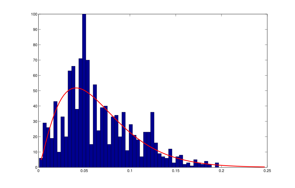
**Figure A1.** Distribution of tariff rates $t(s)$ across 7-digit Taiwanese manufacturing sectors
## B.4 Bertrand Competition
For this experiment we re-solve the model under the assumption that producers compete by simultaneously choosing prices (Bertrand) rather than simultaneously choosing quantities (Cournot). This changes the model set-up in only one way. The demand elasticity facing producer $i$ in sector $s$ is no longer a harmonic weighted average, of $\theta$ and $\gamma$ but is instead a simple arithmetic weighted average, $\varepsilon_i (s) = \omega_i(s) \theta + \left(1-\omega_i(s)\right) \gamma$. With this specification the results are similar to the benchmark. The Bertrand model implies somewhat lower markup dispersion than the Cournot model but also implies a larger change in markup dispersion when opening to trade --- and hence a larger reduction in misallocation.
One problem with the Bertrand model is that it implies a negative correlation between domestic sectoral concentration and domestic import penetration, i.e., in the Bertrand model highly concentrated sectors tend to have low import penetration, the opposite of what we see in the data.
## B.5 Role Of $\gamma$
For our benchmark calibration procedure we obtain $\gamma=10.5$. To see what features of the data determine this value, we have recalibrated our model with a range of alternate values for $\gamma$.
For example, with a much lower value of $\gamma=5$ we find that the model cannot produce a trade elasticity of 4 --- even setting $\rho=0.999$ (effectively perfect correlation) gives a trade elasticity of only 3.59. In addition, as shown in the last few rows of [Table A6](#table:A6), with $\gamma=5$ the model also implies too much intraindustry trade, too little import share dispersion, and too strong an association between sector import shares and size. At the other extreme, with a much higher value of $\gamma=20$, the model can better match the trade elasticity and facts on intraindustry trade and import share dispersion, but now produces too weak an association between sector import shares and size as well as too strong an association between sector concentration and import penetration.
In short, low values like $\gamma=5$ and high values like $\gamma=20$ are at odds with key features of the data. In trying to match these moments, our calibration procedure selects the value $\gamma=10.5$. Importantly, as shown in [Table A7](#table:A7), our model's implications for the gains from trade do not change dramatically even for these extreme values of $\gamma$. For example, with $\gamma=5$ the model implies that the total gains are 16.6% of which 2.7% are pro-competitive gains. With $\gamma=20$ the model implies that total gains are 11.8% of which 1.4% are pro-competitive gains.
## B.6 No Fixed Costs
For this experiment, we solve our model assuming that fixed costs are zero, $f_d=f_x=0$. In this version of the model, all producers operate in both markets. Thus the number of domestic producers in each country in sector $s$ is just given by the geometric draw $n(s)$ for that sector.
As shown in [Table A7](#table:A7), this version of the model yields almost identical gains from trade as the benchmark. Shutting down these extensive margins makes little difference because the typical firm near the margin of operating or not is very small and has negligible impact on the aggregate outcomes.
## B.7 Gaussian Copula
For this experiment we resolve the model using a Gaussian copula to model the cross-country correlation in sectoral productivity draws, specifically $$\tag{46} \mathcal{C}(u,u^*) = \Phi_{2,r} (\Phi^{-1}(u),\Phi^{-1}(u^*))$$ where $\Phi(x)$ denotes the CDF of the standard normal distribution and $\Phi_{2,r}(x,x^*)$ denotes the standard bivariate normal distribution with *linear* correlation coefficient $r\in(-1,1)$. To compare results to the benchmark Gumbel copula, we map the linear correlation coefficient into our preferred Kendall correlation coefficient, which for the Gaussian copula is $\rho=2\arcsin(r)/\pi$. To match a trade elasticity of 4 requires $\rho=0.99$, up from the benchmark 0.94. As shown in [Table A7](#table:A7), this version of the model yields very similar results to our benchmark model. In this sense, the functional form of the copula per se does not seem to matter much for our results, instead, as discussed at length in the main text, it is the amount of correlation $\rho$ in cross-country productivity draws that matters.
## B.8 Uncorrelated $n(s),n^*(s)$
For this experiment, for each sector $s$ we independently draw $n(s)$ producers for the Home country and $n^*(s)$ producers for the Foreign country (each drawn from the same geometric marginal distribution as in the benchmark model). With independent draws for $n(s),n^*(s)$ we find that the model cannot produce a trade elasticity of 4, even setting $\tau(\rho)=0.999$ (effectively perfect correlation) gives a trade elasticity of 2.99. As a consequence of this lower trade elasticity, this version of the model implies very large total gains from trade.
As shown in the last row of [Table A6](#table:A6), with independent draws for $n(s),n^*(s)$ the model implies too strong an association between sector concentration and import penetration relative to the data.
## B.9 5-Digit Sectors
For this last robustness experiment, we recalibrate our model to 5-digit rather than 7-digit data. The second-last column of [Table A6](#table:A6) reports the 5-digit counterparts of our usual 7-digit moments in the Taiwanese data while the last column of [Table A6](#table:A6) reports the model moments when calibrated to this 5-digit data.
At this higher level of aggregation there is less concentration in sectoral shares than there is at the 7-digit level and hence there is less measured misallocation. The productivity losses due to markups are 6.2%, down from the 7% for our benchmark model calibrated to 7-digit data. The total gains from trade remain about the same as in our benchmark but since there is less measured misallocation, the pro-competitive effects are weaker, contributing 0.5% down from our benchmark 2%. Thus, consistent with our earlier results, we see that the pro-competitive gains from trade are smaller when product market distortions are small.
To maintain comparability with our other results, for this experiment we have kept the across-sector elasticity fixed at $\theta=1.24$, which is arguably quite high for 5-digit data.[^20] With a lower value for $\theta$ (e.g., with Cobb-Douglas $\theta=1$) measured misallocation is higher and the pro-competitive gains from trade are correspondingly higher also.
## B.10 Experiments with $N$ Competitors per Sector
To further highlight the role of cross-country correlation in sectoral productivity draws, we have solved a simplified version of our model with the following structure: a fixed number of producers $N$ per sector (the same in both countries), no fixed costs of operating (so all $N$ producers operate), and either perfectly dependent cross-country draws $\rho=1$ or perfectly independent cross-country draws, $\rho=0$. We compare autarky to *free trade* --- i.e., no net trade costs, $\tau=1$, and no fixed costs of exporting $f_x=0$.
Panel A of [Table A8](#table:A8) shows results for the case of *no idiosyncratic* productivity draws, $x_i(s)=1$ for all $i,s$. Now consider the case $N=1$, so that under autarky there is a single monopolist in each sector. In this case there is no misallocation in autarky (there is neither within-sector nor across-sector markup dispersion). Now with free trade there are two producers in each sector (in this sense, it is as if the country size doubles). The effects on misallocation now crucially depend on the cross-country correlation in sectoral productivity. If sectoral productivity draws are independent across countries, then typically one producer gains market share at the expense of the other, and, crucially, this pattern varies across sectors depending on the particular pairs of productivity draws. This creates markup dispersion and hence with free trade there is misallocation whereas there was no misallocation in autarky. Thus the gains from trade will be less than if markups were constant (i.e., aggregate productivity increases by less than first-best productivity). By contrast, if sectoral productivity draws are perfectly correlated across countries, then the two producers (who have equal productivity) split the market between them and this happens exactly the same way in each sector, hence in this case trade does not lead to misallocation. Put differently, $\rho=1$ perfectly *mitigates* the increase in misallocation that would otherwise happen.
+:-----------+:----------------------------------------------------------+:----------:+:------------:+:-----------:+:-----------+:-------------------+:----------:+:------------:+:-----------:+
| Panel A: No Idiosyncratic Productivity Draws |
+------------+-----------------------------------------------------------+------------+----------------------------+------------+--------------------+------------+----------------------------+
| | | | Free trade | | | | Free trade |
+------------+-----------------------------------------------------------+------------+--------------+-------------+------------+--------------------+------------+--------------+-------------+
| | | Autarky | $\rho = 1$ | $\rho = 0$ | | | Autarky | $\rho = 1$ | $\rho = 0$ |
+------------+-----------------------------------------------------------+------------+--------------+-------------+------------+--------------------+------------+--------------+-------------+
| $N=1$ | | | | | $N=2$ | | | | |
+------------+-----------------------------------------------------------+------------+--------------+-------------+------------+--------------------+------------+--------------+-------------+
| | TFP loss, % | 0 | 0 | 16.4 | | TFP loss, % | 0 | 0 | 0.9 |
+------------+-----------------------------------------------------------+------------+--------------+-------------+------------+--------------------+------------+--------------+-------------+
| | import share | 0 | 0.5 | 0.5 | | import share | 0 | 0.5 | 0.5 |
+------------+-----------------------------------------------------------+------------+--------------+-------------+------------+--------------------+------------+--------------+-------------+
| | fraction exporters | 0 | 1 | 1 | | fraction exporters | 0 | 1 | 1 |
+------------+-----------------------------------------------------------+------------+--------------+-------------+------------+--------------------+------------+--------------+-------------+
| | trade elasticity | | 1.32 | 0.56 | | trade elasticity | | 2.85 | 0.63 |
+------------+-----------------------------------------------------------+------------+--------------+-------------+------------+--------------------+------------+--------------+-------------+
| | aggregate markup | 5.25 | 1.83 | 3.48 | | aggregate markup | 1.83 | 1.38 | 1.76 |
+------------+-----------------------------------------------------------+------------+--------------+-------------+------------+--------------------+------------+--------------+-------------+
| | domestic markup | 5.25 | 1.83 | 3.48 | | domestic markup | 1.83 | 1.38 | 1.76 |
+------------+-----------------------------------------------------------+------------+--------------+-------------+------------+--------------------+------------+--------------+-------------+
| | import markup | | 1.83 | 3.48 | | import markup | | 1.38 | 1.76 |
+------------+-----------------------------------------------------------+------------+--------------+-------------+------------+--------------------+------------+--------------+-------------+
| | Markup dispersion | | | | | Markup dispersion | | | |
+------------+-----------------------------------------------------------+------------+--------------+-------------+------------+--------------------+------------+--------------+-------------+
| | unconditional | 0 | 0 | 0.59 | | unconditional | 0 | 0 | 0.22 |
+------------+-----------------------------------------------------------+------------+--------------+-------------+------------+--------------------+------------+--------------+-------------+
| | sectoral | 0 | 0 | 0 | | sectoral | 0 | 0 | 0 |
+------------+-----------------------------------------------------------+------------+--------------+-------------+------------+--------------------+------------+--------------+-------------+
| $N=10$ | | | | | $N=20$ | | | | |
+------------+-----------------------------------------------------------+------------+--------------+-------------+------------+--------------------+------------+--------------+-------------+
| | TFP loss, % | 0 | 0 | 0.02 | | TFP loss, % | 0 | 0 | 0.004 |
+------------+-----------------------------------------------------------+------------+--------------+-------------+------------+--------------------+------------+--------------+-------------+
| | import share | 0 | 0.5 | 0.5 | | import share | 0 | 0.5 | 0.5 |
+------------+-----------------------------------------------------------+------------+--------------+-------------+------------+--------------------+------------+--------------+-------------+
| | fraction exporters | 0 | 1 | 1 | | fraction exporters | 0 | 1 | 1 |
+------------+-----------------------------------------------------------+------------+--------------+-------------+------------+--------------------+------------+--------------+-------------+
| | trade elasticity | | 6.83 | 0.71 | | trade elasticity | | 7.97 | 0.66 |
+------------+-----------------------------------------------------------+------------+--------------+-------------+------------+--------------------+------------+--------------+-------------+
| | aggregate markup | 1.20 | 1.15 | 1.20 | | aggregate markup | 1.15 | 1.13 | 1.15 |
+------------+-----------------------------------------------------------+------------+--------------+-------------+------------+--------------------+------------+--------------+-------------+
| | domestic markup | 1.20 | 1.15 | 1.20 | | domestic markup | 1.15 | 1.13 | 1.15 |
+------------+-----------------------------------------------------------+------------+--------------+-------------+------------+--------------------+------------+--------------+-------------+
| | import markup | | 1.15 | 1.20 | | import markup | | 1.13 | 1.15 |
+------------+-----------------------------------------------------------+------------+--------------+-------------+------------+--------------------+------------+--------------+-------------+
| | Markup dispersion | | | | | Markup dispersion | | | |
+------------+-----------------------------------------------------------+------------+--------------+-------------+------------+--------------------+------------+--------------+-------------+
| | unconditional | 0 | 0 | 0.04 | | unconditional | 0 | 0 | 0.02 |
+------------+-----------------------------------------------------------+------------+--------------+-------------+------------+--------------------+------------+--------------+-------------+
| | sectoral | 0 | 0 | 0 | | sectoral | 0 | 0 | 0 |
+------------+-----------------------------------------------------------+------------+--------------+-------------+------------+--------------------+------------+--------------+-------------+
| Panel B: With Idiosyncratic Productivity Draws |
+------------+-----------------------------------------------------------+------------+----------------------------+------------+--------------------+------------+----------------------------+
| | | | Free trade | | | | Free trade |
+------------+-----------------------------------------------------------+------------+--------------+-------------+------------+--------------------+------------+--------------+-------------+
| | | Autarky | $\rho = 1$ | $\rho = 0$ | | | Autarky | $\rho = 1$ | $\rho = 0$ |
+------------+-----------------------------------------------------------+------------+--------------+-------------+------------+--------------------+------------+--------------+-------------+
| $N=1$ | | | | | $N=2$ | | | | |
+------------+-----------------------------------------------------------+------------+--------------+-------------+------------+--------------------+------------+--------------+-------------+
| | TFP loss, % | 0 | 4.6 | 15.9 | | TFP loss, % | 4.25 | 6.73 | 6.01 |
+------------+-----------------------------------------------------------+------------+--------------+-------------+------------+--------------------+------------+--------------+-------------+
| | import share | 0 | 0.5 | 0.5 | | import share | 0 | 0.5 | 0.5 |
+------------+-----------------------------------------------------------+------------+--------------+-------------+------------+--------------------+------------+--------------+-------------+
| | fraction exporters | 0 | 1 | 1 | | fraction exporters | 0 | 1 | 1 |
+------------+-----------------------------------------------------------+------------+--------------+-------------+------------+--------------------+------------+--------------+-------------+
| | trade elasticity | | 1.29 | 0.55 | | trade elasticity | | 2.60 | 0.62 |
+------------+-----------------------------------------------------------+------------+--------------+-------------+------------+--------------------+------------+--------------+-------------+
| | aggregate markup | 5.25 | 1.88 | 3.55 | | aggregate markup | 1.87 | 1.47 | 1.80 |
+------------+-----------------------------------------------------------+------------+--------------+-------------+------------+--------------------+------------+--------------+-------------+
| | domestic markup | 5.25 | 1.88 | 3.55 | | domestic markup | 1.87 | 1.47 | 1.80 |
+------------+-----------------------------------------------------------+------------+--------------+-------------+------------+--------------------+------------+--------------+-------------+
| | import markup | | 1.88 | 3.55 | | import markup | | 1.47 | 1.80 |
+------------+-----------------------------------------------------------+------------+--------------+-------------+------------+--------------------+------------+--------------+-------------+
| | Markup dispersion | | | | | Markup dispersion | | | |
+------------+-----------------------------------------------------------+------------+--------------+-------------+------------+--------------------+------------+--------------+-------------+
| | unconditional | 0 | 0.14 | 0.59 | | unconditional | 0.13 | 0.14 | 0.24 |
+------------+-----------------------------------------------------------+------------+--------------+-------------+------------+--------------------+------------+--------------+-------------+
| | sectoral | 0 | 0 | 0 | | sectoral | 0.06 | 0.09 | 0.12 |
+------------+-----------------------------------------------------------+------------+--------------+-------------+------------+--------------------+------------+--------------+-------------+
| $N=10$ | | | | | $N=20$ | | | | |
+------------+-----------------------------------------------------------+------------+--------------+-------------+------------+--------------------+------------+--------------+-------------+
| | TFP loss, % | 8.0 | 7.8 | 8.3 | | TFP loss, % | 7.4 | 7.1 | 10.5 |
+------------+-----------------------------------------------------------+------------+--------------+-------------+------------+--------------------+------------+--------------+-------------+
| | import share | 0 | 0.5 | 0.5 | | import share | 0 | 0.5 | 0.5 |
+------------+-----------------------------------------------------------+------------+--------------+-------------+------------+--------------------+------------+--------------+-------------+
| | fraction exporters | 0 | 1 | 1 | | fraction exporters | 0 | 1 | 1 |
+------------+-----------------------------------------------------------+------------+--------------+-------------+------------+--------------------+------------+--------------+-------------+
| | trade elasticity | | 4.33 | 0.65 | | trade elasticity | | 4.67 | 0.65 |
+------------+-----------------------------------------------------------+------------+--------------+-------------+------------+--------------------+------------+--------------+-------------+
| | aggregate markup | 1.33 | 1.31 | 1.34 | | aggregate markup | 1.30 | 1.28 | 1.35 |
+------------+-----------------------------------------------------------+------------+--------------+-------------+------------+--------------------+------------+--------------+-------------+
| | domestic markup | 1.33 | 1.31 | 1.34 | | domestic markup | 1.30 | 1.28 | 1.35 |
+------------+-----------------------------------------------------------+------------+--------------+-------------+------------+--------------------+------------+--------------+-------------+
| | import markup | | 1.31 | 1.34 | | import markup | | 1.28 | 1.35 |
+------------+-----------------------------------------------------------+------------+--------------+-------------+------------+--------------------+------------+--------------+-------------+
| | Markup dispersion | | | | | Markup dispersion | | | |
+------------+-----------------------------------------------------------+------------+--------------+-------------+------------+--------------------+------------+--------------+-------------+
| | unconditional | 0.11 | 0.08 | 0.09 | | unconditional | 0.08 | 0.06 | 0.06 |
+------------+-----------------------------------------------------------+------------+--------------+-------------+------------+--------------------+------------+--------------+-------------+
| | sectoral | 0.10 | 0.11 | 0.11 | | sectoral | 0.12 | 0.12 | 0.12 |
+------------+-----------------------------------------------------------+------------+--------------+-------------+------------+--------------------+------------+--------------+-------------+
| | Notes: | | | | | | | | |
+------------+-----------------------------------------------------------+------------+--------------+-------------+------------+--------------------+------------+--------------+-------------+
| | N is number of producers per sector per country | | | | | | | | |
+------------+-----------------------------------------------------------+------------+--------------+-------------+------------+--------------------+------------+--------------+-------------+
| | No fixed cost of operating, $f_d=0$ | | | | | | | | |
+------------+-----------------------------------------------------------+------------+--------------+-------------+------------+--------------------+------------+--------------+-------------+
| | Free trade means $\tau=1$ (no net trade cost) and $f_x=0$ | | | | | | | | |
+------------+-----------------------------------------------------------+------------+--------------+-------------+------------+--------------------+------------+--------------+-------------+
| | Markup dispersion is measured as std dev of log markups | | | | | | | | |
+------------+-----------------------------------------------------------+------------+--------------+-------------+------------+--------------------+------------+--------------+-------------+
: **Table A8.** Fixed N Experiments
Notice that the extent of misallocation created when sectoral productivity draws are independent is *decreasing* in $N$ --- and steeply decreasing in $N$ at that. With independent draws and $N=1$, free trade creates productivity losses of 16.4% relative to the first-best, with $N=2$ the losses are much smaller, 0.9% and with $N=10$ the losses are down to 0.02%.
Panel B of [Table A8](#table:A8) shows the same exercise but now *with idiosyncratic* productivity draws, as in the benchmark model. We again see that for low $N$ opening to trade creates misallocation and that this misallocation is mitigated by correlated sectoral productivity draws. By the time we get to $N=10$ (which is similar to our benchmark model, which has a median of about 10 producers per sector per country), opening to free trade reduces misallocation if sectoral draws are correlated.
# C Extensions
Our benchmark model makes several stark simplifying assumptions: (i) labor is the only factor of production and is in inelastic supply, (ii) the two countries Home and Foreign are symmetric at the aggregate level, and (iii) there is an exogenous number of competitors per sector. Here we provide further details on extensions of our benchmark model that relax these assumptions. Since the main text already discusses the results from these extensions at some length, here we focus on recording additional details that were omitted from the main text to save space.
## C.1 Capital Accumulation and Elastic Labor Supply
In the benchmark model, the only source of pro-competitive gains from trade is changes in markup *dispersion*. Changes in the *level* of the aggregate markup $\mu$ have no welfare implications. But with capital accumulation and/or elastic labor supply, the aggregate markup $\mu$ acts like a distortionary wedge affecting investment and labor supply decisions, and, because of this, a reduction in the aggregate markup increases welfare beyond the increases associated with a reduction in markup dispersion.
**Setup.** To illustrate this, we solve a simple dynamic extension of our benchmark model. Specifically, we suppose the representative consumer has intertemporal preferences $\sum_{t=0}^{\infty} \beta^t U(C_t,L_t)$ over aggregate consumption $C_t$ and labor $L_t$, that capital is accumulated according to $K_{t+1}=(1-\delta)K_t + I_t$, and that individual producers have production function $y=a k^{\alpha} l^{1-\alpha}$. We then have a standard two-country representative consumer economy with aggregate production function $Y_t = A_t K_t^{\alpha}\tilde{L}_t^{1-\alpha}$ where $A_t$ is aggregate productivity (TFP) as in the main text and where $\tilde{L}_t$ is aggregate employment net of fixed costs.
**Aggregate markup distortions.** Using the representative consumer's optimality conditions for capital accumulation and labor supply and the firms' optimal input demands gives the equilibrium conditions $$\tag{47} U_{c,t} = \beta U_{c,t+1} \Big(\frac{1}{\mu_{t+1}}\alpha\frac{Y_{t+1}}{K_{t+1}} + 1-\delta \Big)\, ,$$ and $$\tag{48} -\frac{U_{l,t}}{U_{c,t}} = \frac{W_t}{P_t} = \frac{1}{\mu_t}(1-\alpha)\frac{Y_t}{\tilde{L}_t}\, ,$$ where $\mu_t$ is the aggregate markup as in the main text. High aggregate markups thus act like distortionary capital and labor income taxes and reduce output relative to its efficient level.
**Parameterization.** To quantify the additional welfare effects of changes in the aggregate markup, we solve this version of the model assuming utility function $U(C,L)=\log C - L^{1+\eta}/{1+\eta}$ and assuming discount factor $\beta=0.96$, depreciation rate $\delta=0.1$ and output elasticity of capital $\alpha=1/3$. We report results for various elasticities of labor supply $\eta$. We start the economy in autarky and then compute the transition to a new steady-state corresponding to the Taiwan benchmark. We measure the welfare gains as the consumption compensating variation taking into account the dynamics of consumption and employment during the transition to the new steady-state.
**Results.** The first column of [Table A9](#table:A9) shows what happens in a standard model with constant markups if TFP increases by 10.4%, i.e., the benchmark increase in first-best TFP. Physical capital, output, and consumption all increase by 15.7%, i.e., by $1/(1-\alpha)=1.5$ times the increase in TFP. Aggregate labor does not change because utility is log in consumption so that the income and substitution effects implied by the change in TFP exactly cancel out. The measured welfare gain is slightly less than the long-run increase in aggregate consumption because we take the transitional dynamics into account.
+--------------------------+------------------------------+----------------+--------------------------------------------------------------------------------------------+
| | | | Variable markups |
+--------------------------+------------------------------+----------------+-----------------+--------------------------------------------------------------------------+
| | | | Aggregate | Frisch elasticity of labor supply ($1/\eta$) |
+--------------------------+------------------------------+----------------+-----------------+--------------+--------------+--------------+--------------+--------------+
| | | Standard model | markup constant | 0 | 0.5 | 1 | 2 | $\infty$ |
+:=========================+:=============================+:==============:+:===============:+:============:+:============:+:============:+:============:+:============:+
| change TFP, % | | 10.4 | 12.4 | 12.4 | 12.4 | 12.4 | 12.4 | 12.4 |
+--------------------------+------------------------------+----------------+-----------------+--------------+--------------+--------------+--------------+--------------+
| change markup, % | | 0 | 0 | -2.9 | -2.9 | -2.9 | -2.9 | -2.9 |
+--------------------------+------------------------------+----------------+-----------------+--------------+--------------+--------------+--------------+--------------+
| change C, % | | 15.7 | 18.6 | 19.5 | 20.7 | 21.2 | 21.8 | 23.0 |
+--------------------------+------------------------------+----------------+-----------------+--------------+--------------+--------------+--------------+--------------+
| change K, % | | 15.7 | 18.6 | 23.0 | 24.2 | 24.8 | 25.4 | 26.6 |
+--------------------------+------------------------------+----------------+-----------------+--------------+--------------+--------------+--------------+--------------+
| change Y, % | | 15.7 | 18.6 | 20.1 | 21.3 | 21.9 | 22.5 | 23.7 |
+--------------------------+------------------------------+----------------+-----------------+--------------+--------------+--------------+--------------+--------------+
| change L, % | | 0 | 0 | 0 | 1.2 | 1.8 | 2.4 | 3.6 |
+--------------------------+------------------------------+----------------+-----------------+--------------+--------------+--------------+--------------+--------------+
| change welfare, % | | 14.5 | 16.9 | 18.0 | 18.1 | 18.1 | 18.2 | 18.4 |
+--------------------------+------------------------------+----------------+-----------------+--------------+--------------+--------------+--------------+--------------+
| *(including transition)* |
+--------------------------+------------------------------+----------------+-----------------+--------------+--------------+--------------+--------------+--------------+
| pro-competitive gains, % | | 0 | 2.4 | 3.5 | 3.6 | 3.6 | 3.7 | 3.9 |
+--------------------------+------------------------------+----------------+-----------------+--------------+--------------+--------------+--------------+--------------+
| *Other parameters:* |
+--------------------------+------------------------------+----------------+-----------------+--------------+--------------+--------------+--------------+--------------+
| $\alpha$ | output elasticity of capital | 0.33 | | | | | | |
+--------------------------+------------------------------+----------------+-----------------+--------------+--------------+--------------+--------------+--------------+
| $\beta$ | time discount factor | 0.96 | | | | | | |
+--------------------------+------------------------------+----------------+-----------------+--------------+--------------+--------------+--------------+--------------+
| $\delta$ | capital depreciation rate | 0.1 | | | | | | |
+--------------------------+------------------------------+----------------+-----------------+--------------+--------------+--------------+--------------+--------------+
: **Table A9.** Gains from Trade with Capital Accumulation and Elastic Labor Supply
The next column shows the corresponding results in our model with variable markups but where we hold the aggregate markup unchanged. Thus TFP increases by 12.4% because in addition to the first-best 10.4% there are now pro-competitive gains of 2%. Aggregate labor is again constant because of log utility and because the aggregate markup is held fixed. Thus the additional gains here are entirely because capital accumulation magnifies the TFP gains.
The remaining columns show results when we also allow the aggregate markup to change, falling by $2.9\%$ from autarky to the new steady-state. We report results for various choices of the Frisch elasticity of labor supply $1/\eta$. If labor supply is inelastic, so the fall in the aggregate markup affects capital accumulation alone, welfare increases by 18%. This gain is larger than the 17% we had when only TFP changes and the additional gain of 1% is entirely due to the effect of the change in the aggregate markup and hence this extra 1% is entirely due to pro-competitive effects, making for a total pro-competitive gain of 3.5%. Elastic labor supply magnifies these gains yet further. With a Frisch elasticity of 1, the pro-competitive gains rise to 3.6% (as shown in [Table A9](#table:A9), the size of the pro-competitive gains are not sensitive to a Frisch elasticity in the range 0.5 to 2). In short, we see that with elastic factor supply the relative importance of the pro-competitive effects is larger than in our benchmark model.
## C.2 Asymmetric Countries
Our benchmark model assumes trade between two symmetric countries. We now relax this and consider trade between countries that differ in size and/or productivity.
**Setup.** Let $L,L^*$ denote Home and Foreign labor forces and let $\bar{A},\bar{A}^*$ denote Home and Foreign economy-wide productivity --- that is, Home producers now have technology $y_i(s) = \bar{A} a_i(s)l_i(s)$ and Foreign producers have $y^*_i(s)=\bar{A}^* a_i^*(s)l_i^*(s)$. We normalize $L=1$ and $\bar{A}=1$ and consider various $L^*$ and $\bar{A}^*$.
In our benchmark model, aggregate symmetry implied that the wage in each country was the same so that by choosing the Home wage as numeraire we simply had $W=W^*=1$ along with symmetric price levels $P=P^*$ and symmetric productivities $A=A^*$ so that the real wage in both countries was $1/P$ and the aggregate (economy-wide) markup in both countries was $\mu = PA$.
We continue to choose the Home country wage as numeraire, $W=1$, but with asymmetric countries now have to solve for the Foreign wage $W^*$ in equilibrium. Intuitively, $W^*$ has to adjust to ensure that trade between the two countries is balanced. With asymmetric countries, the equilibrium price levels $P,P^*$ and aggregate productivities $A,A^*$ likewise differ across countries. We then have Home real wage $1/P$ and aggregate markup $\mu=PA$ and Foreign real wage $W^*/P^*$ and aggregate markup $\mu^*=P^* A^*/W^*$.
**Parameterization.** We consider $L^*=2$ and $L^*=10$ times as large as Home, holding economy-wide productivity the same in both countries, and then consider $\bar{A}^*=2$ and $\bar{A}^*=10$ times as great as Home productivity, now holding the labor force the same in both countries. For each of these four experiments, we recalibrate the model so that, *for the Home country*, we reproduce the degree of openness of the Taiwan benchmark --- in particular, we choose the proportional trade cost $\tau$, export fixed cost $f_x$, and correlation parameter $\rho$ so that the Home country continues to have an aggregate import share of 0.38, fraction of exporters 0.25 and trade elasticity $4$. [Table A10](#table:A10) reports the full set of parameters used for each experiment, [Table A11](#table:A11) reports the target moments and their model counterparts for both Home and Foreign countries for each experiment, and [Table A12](#table:A12) reports the gains from trade and statistics on markup dispersion for both Home and Foreign countries for each experiment. In addition to our usual aggregate statistics, in [Table A12](#table:A12) we also report the relative real wage expressed as the real wage of Foreign to Home, that is $(W^*/P^*)/(W/P) = (A^*/A)/(\mu^*/\mu)$.
+-----------+----------------------------------------------------+-----------+---------------------------+----------------------------------------------+
| | | | Larger trading partner | More productive trading partner |
+-----------+----------------------------------------------------+-----------+-------------+-------------+----------------------+-----------------------+
| | | Benchmark | $L^*=2L$ | $L^*=10L$ | $\bar{A}^*=2\bar{A}$ | $\bar{A}^*=10\bar{A}$ |
+:==========+:===================================================+:=========:+:===========:+:===========:+:====================:+:=====================:+
| $\gamma$ | within-sector elasticity of substitution | 10.5 | 10.5 | 10.5 | 10.2 | 10.2 |
+-----------+----------------------------------------------------+-----------+-------------+-------------+----------------------+-----------------------+
| $\theta$ | across-sector elasticity of substitution | 1.24 | 1.24 | 1.24 | 1.23 | 1.23 |
+-----------+----------------------------------------------------+-----------+-------------+-------------+----------------------+-----------------------+
| $\xi_{x}$ | pareto shape parameter, idiosyncratic productivity | 4.58 | 4.58 | 4.58 | 4.58 | 4.58 |
+-----------+----------------------------------------------------+-----------+-------------+-------------+----------------------+-----------------------+
| $\xi_{z}$ | pareto shape parameter, sector productivity | 0.51 | 0.51 | 0.51 | 0.51 | 0.51 |
+-----------+----------------------------------------------------+-----------+-------------+-------------+----------------------+-----------------------+
| $\zeta$ | geometric parameter, number producers per sector | 0.043 | 0.043 | 0.043 | 0.043 | 0.043 |
+-----------+----------------------------------------------------+-----------+-------------+-------------+----------------------+-----------------------+
| $f_{d}$ | fixed cost of domestic operations | 0.004 | 0.004 | 0.004 | 0.004 | 0.004 |
+-----------+----------------------------------------------------+-----------+-------------+-------------+----------------------+-----------------------+
| $f_{x}$ | fixed cost of export operations | 0.203 | 0.203 | 0.203 | 0.250 | 0.300 |
+-----------+----------------------------------------------------+-----------+-------------+-------------+----------------------+-----------------------+
| $\tau$ | trade cost | 1.129 | 1.245 | 1.500 | 1.132 | 2.660 |
+-----------+----------------------------------------------------+-----------+-------------+-------------+----------------------+-----------------------+
| $\rho$ | kendall correlation | 0.94 | 0.94 | 0.96 | 0.86 | 0.60 |
+-----------+----------------------------------------------------+-----------+-------------+-------------+----------------------+-----------------------+
: **Table A10.** Parameters for Asymmetric Countries Experiments
+-------------------------------------------+--------------+--------------+--------------+-----------------------------------------------------------+-----------------------------------------------------------+
| | | | | Larger trading partner | More productive trading partner |
+-------------------------------------------+--------------+--------------+--------------+-----------------------------+-----------------------------+-----------------------------+-----------------------------+
| | | Benchmark | $L^*=2L$ | $L^*=10L$ | $\bar{A}^*=2\bar{A}$ | $\bar{A}^*=10\bar{A}$ |
+-------------------------------------------+--------------+--------------+--------------+--------------+--------------+--------------+--------------+--------------+--------------+--------------+--------------+
| | Data | Home | Foreign | Home | Foreign | Home | Foreign | Home | Foreign | Home | Foreign |
+:==========================================+:============:+:============:+:============:+:============:+:============:+:============:+:============:+:============:+:============:+:============:+:============:+
| *Within-sector concentration, domestic sales* |
+-------------------------------------------+--------------+--------------+--------------+--------------+--------------+--------------+--------------+--------------+--------------+--------------+--------------+
| mean inverse HH | 7.25 | 4.30 | 4.30 | 4.29 | 16.63 | 4.28 | 17.08 | 4.36 | 16.70 | 4.46 | 17.14 |
+-------------------------------------------+--------------+--------------+--------------+--------------+--------------+--------------+--------------+--------------+--------------+--------------+--------------+
| median inverse HH | 3.92 | 3.79 | 3.79 | 3.79 | 4.48 | 3.77 | 4.93 | 3.81 | 4.52 | 3.86 | 4.93 |
+-------------------------------------------+--------------+--------------+--------------+--------------+--------------+--------------+--------------+--------------+--------------+--------------+--------------+
| mean top share | 0.45 | 0.46 | 0.46 | 0.46 | 0.40 | 0.46 | 0.37 | 0.46 | 0.40 | 0.47 | 0.38 |
+-------------------------------------------+--------------+--------------+--------------+--------------+--------------+--------------+--------------+--------------+--------------+--------------+--------------+
| median top share | 0.40 | 0.41 | 0.41 | 0.41 | 0.37 | 0.41 | 0.34 | 0.41 | 0.36 | 0.40 | 0.34 |
+-------------------------------------------+--------------+--------------+--------------+--------------+--------------+--------------+--------------+--------------+--------------+--------------+--------------+
| *Distribution of sectoral shares, domestic sales* |
+-------------------------------------------+--------------+--------------+--------------+--------------+--------------+--------------+--------------+--------------+--------------+--------------+--------------+
| mean share | 0.04 | 0.05 | 0.05 | 0.05 | 0.03 | 0.05 | 0.03 | 0.05 | 0.03 | 0.05 | 0.03 |
+-------------------------------------------+--------------+--------------+--------------+--------------+--------------+--------------+--------------+--------------+--------------+--------------+--------------+
| median share | 0.005 | 0.005 | 0.005 | 0.005 | 0.004 | 0.005 | 0.004 | 0.006 | 0.004 | 0.007 | 0.004 |
+-------------------------------------------+--------------+--------------+--------------+--------------+--------------+--------------+--------------+--------------+--------------+--------------+--------------+
| p75 share | 0.02 | 0.03 | 0.03 | 0.03 | 0.01 | 0.03 | 0.01 | 0.03 | 0.01 | 0.04 | 0.01 |
+-------------------------------------------+--------------+--------------+--------------+--------------+--------------+--------------+--------------+--------------+--------------+--------------+--------------+
| p95 share | 0.19 | 0.27 | 0.27 | 0.27 | 0.17 | 0.27 | 0.16 | 0.27 | 0.16 | 0.28 | 0.16 |
+-------------------------------------------+--------------+--------------+--------------+--------------+--------------+--------------+--------------+--------------+--------------+--------------+--------------+
| p99 share | 0.59 | 0.59 | 0.59 | 0.59 | 0.45 | 0.58 | 0.41 | 0.61 | 0.45 | 0.65 | 0.42 |
+-------------------------------------------+--------------+--------------+--------------+--------------+--------------+--------------+--------------+--------------+--------------+--------------+--------------+
| std dev share | 0.11 | 0.12 | 0.12 | 0.12 | 0.09 | 0.11 | 0.08 | 0.12 | 0.09 | 0.12 | 0.08 |
+-------------------------------------------+--------------+--------------+--------------+--------------+--------------+--------------+--------------+--------------+--------------+--------------+--------------+
| *Across-sector concentration* |
+-------------------------------------------+--------------+--------------+--------------+--------------+--------------+--------------+--------------+--------------+--------------+--------------+--------------+
| p10 inverse HH | 1.17 | 1.70 | 1.70 | 1.71 | 1.98 | 1.71 | 2.00 | 1.56 | 1.92 | 1.18 | 1.98 |
+-------------------------------------------+--------------+--------------+--------------+--------------+--------------+--------------+--------------+--------------+--------------+--------------+--------------+
| p50 inverse HH | 3.73 | 3.79 | 3.79 | 3.79 | 4.51 | 3.77 | 4.95 | 3.81 | 4.56 | 3.86 | 4.95 |
+-------------------------------------------+--------------+--------------+--------------+--------------+--------------+--------------+--------------+--------------+--------------+--------------+--------------+
| p90 inverse HH | 13.82 | 7.66 | 7.66 | 7.61 | 9.77 | 7.55 | 10.56 | 7.93 | 10.29 | 8.38 | 10.86 |
+-------------------------------------------+--------------+--------------+--------------+--------------+--------------+--------------+--------------+--------------+--------------+--------------+--------------+
| p10 top share | 0.16 | 0.24 | 0.24 | 0.24 | 0.19 | 0.24 | 0.18 | 0.23 | 0.18 | 0.22 | 0.18 |
+-------------------------------------------+--------------+--------------+--------------+--------------+--------------+--------------+--------------+--------------+--------------+--------------+--------------+
| p50 top share | 0.41 | 0.41 | 0.41 | 0.41 | 0.37 | 0.41 | 0.34 | 0.41 | 0.36 | 0.40 | 0.34 |
+-------------------------------------------+--------------+--------------+--------------+--------------+--------------+--------------+--------------+--------------+--------------+--------------+--------------+
| p90 top share | 0.92 | 0.75 | 0.75 | 0.75 | 0.65 | 0.74 | 0.59 | 0.79 | 0.68 | 0.92 | 0.62 |
+-------------------------------------------+--------------+--------------+--------------+--------------+--------------+--------------+--------------+--------------+--------------+--------------+--------------+
| p10 number producers | 2 | 3 | 3 | 3 | 3 | 3 | 3 | 3 | 3 | 2 | 3 |
+-------------------------------------------+--------------+--------------+--------------+--------------+--------------+--------------+--------------+--------------+--------------+--------------+--------------+
| p50 number producers | 10 | 16 | 16 | 16 | 18 | 16 | 18 | 15 | 17 | 13 | 18 |
+-------------------------------------------+--------------+--------------+--------------+--------------+--------------+--------------+--------------+--------------+--------------+--------------+--------------+
| p90 number producers | 52 | 47 | 47 | 48 | 64 | 48 | 68 | 46 | 64 | 46 | 66 |
+-------------------------------------------+--------------+--------------+--------------+--------------+--------------+--------------+--------------+--------------+--------------+--------------+--------------+
| *Size distribution sectors, domestic sales* |
+-------------------------------------------+--------------+--------------+--------------+--------------+--------------+--------------+--------------+--------------+--------------+--------------+--------------+
| fraction sales by top 0.01 sectors | 0.26 | 0.21 | 0.21 | 0.21 | 0.21 | 0.21 | 0.21 | 0.21 | 0.21 | 0.21 | 0.20 |
+-------------------------------------------+--------------+--------------+--------------+--------------+--------------+--------------+--------------+--------------+--------------+--------------+--------------+
| fraction sales by top 0.05 sectors | 0.52 | 0.32 | 0.32 | 0.32 | 0.32 | 0.32 | 0.31 | 0.33 | 0.32 | 0.34 | 0.30 |
+-------------------------------------------+--------------+--------------+--------------+--------------+--------------+--------------+--------------+--------------+--------------+--------------+--------------+
| fraction wages (same) top 0.01 sectors | 0.11 | 0.22 | 0.22 | 0.22 | 0.22 | 0.22 | 0.22 | 0.22 | 0.22 | 0.23 | 0.22 |
+-------------------------------------------+--------------+--------------+--------------+--------------+--------------+--------------+--------------+--------------+--------------+--------------+--------------+
| fraction wages (same) top 0.05 sectors | 0.32 | 0.33 | 0.33 | 0.33 | 0.33 | 0.33 | 0.33 | 0.34 | 0.33 | 0.35 | 0.32 |
+-------------------------------------------+--------------+--------------+--------------+--------------+--------------+--------------+--------------+--------------+--------------+--------------+--------------+
| *Size distribution producers, domestic sales* |
+-------------------------------------------+--------------+--------------+--------------+--------------+--------------+--------------+--------------+--------------+--------------+--------------+--------------+
| fraction sales by top 0.01 producers | 0.41 | 0.33 | 0.33 | 0.33 | 0.38 | 0.33 | 0.36 | 0.33 | 0.37 | 0.31 | 0.36 |
+-------------------------------------------+--------------+--------------+--------------+--------------+--------------+--------------+--------------+--------------+--------------+--------------+--------------+
| fraction sales by top 0.05 producers | 0.65 | 0.61 | 0.61 | 0.61 | 0.69 | 0.62 | 0.67 | 0.61 | 0.69 | 0.58 | 0.67 |
+-------------------------------------------+--------------+--------------+--------------+--------------+--------------+--------------+--------------+--------------+--------------+--------------+--------------+
| fraction wages top 0.01 producers | 0.24 | 0.31 | 0.31 | 0.31 | 0.35 | 0.31 | 0.33 | 0.30 | 0.34 | 0.28 | 0.32 |
+-------------------------------------------+--------------+--------------+--------------+--------------+--------------+--------------+--------------+--------------+--------------+--------------+--------------+
| fraction wages top 0.05 producers | 0.47 | 0.57 | 0.57 | 0.57 | 0.65 | 0.57 | 0.63 | 0.56 | 0.65 | 0.53 | 0.62 |
+-------------------------------------------+--------------+--------------+--------------+--------------+--------------+--------------+--------------+--------------+--------------+--------------+--------------+
| *Import dispersion statistics* |
+-------------------------------------------+--------------+--------------+--------------+--------------+--------------+--------------+--------------+--------------+--------------+--------------+--------------+
| coefficient, share imports on share sales | 0.81 | 0.55 | 0.55 | 0.56 | 0.66 | 0.58 | 0.34 | 0.42 | 0.52 | 0.26 | -0.03 |
+-------------------------------------------+--------------+--------------+--------------+--------------+--------------+--------------+--------------+--------------+--------------+--------------+--------------+
| index import share dispersion | 0.38 | 0.26 | 0.26 | 0.24 | 0.22 | 0.22 | 0.19 | 0.42 | 0.39 | 0.68 | 0.75 |
+-------------------------------------------+--------------+--------------+--------------+--------------+--------------+--------------+--------------+--------------+--------------+--------------+--------------+
| index intraindustry trade | 0.37 | 0.45 | 0.45 | 0.40 | 0.40 | 0.22 | 0.22 | 0.26 | 0.26 | 0.01 | 0.01 |
+-------------------------------------------+--------------+--------------+--------------+--------------+--------------+--------------+--------------+--------------+--------------+--------------+--------------+
: **Table A11.** Moments implied by Asymmetric Countries Experiments
+-------------------------------+-------+---------+---------------------------------------+-----------------------------------------------------+
| | | | Larger trading partner | More productive trading partner |
+-------------------------------+-------+---------+-------------------+-------------------+-------------------------+---------------------------+
| | Benchmark | $L^*=2L$ | $L^*=10L$ | $\bar{A}^*=2\bar{A}$ | $\bar{A}^*=10\bar{A}$ |
+-------------------------------+-------+---------+---------+---------+---------+---------+------------+------------+-------------+-------------+
| | Home | Foreign | Home | Foreign | Home | Foreign | Home | Foreign | Home | Foreign |
+:==============================+:=====:+:=======:+:=======:+:=======:+:=======:+:=======:+:==========:+:==========:+:===========:+:===========:+
| TFP loss autarky, % | 9.0 | 9.0 | 9.0 | 9.0 | 9.0 | 9.0 | 9.0 | 9.0 | 9.0 | 9.0 |
+-------------------------------+-------+---------+---------+---------+---------+---------+------------+------------+-------------+-------------+
| TFP loss, % | 7.0 | 7.0 | 7.3 | 6.8 | 7.1 | 7.5 | 7.4 | 7.0 | 7.5 | 8.6 |
+-------------------------------+-------+---------+---------+---------+---------+---------+------------+------------+-------------+-------------+
| gains from trade, % | 12.4 | 12.4 | 12.0 | 6.5 | 12.0 | 2.2 | 15.3 | 8.1 | 31.9 | 5.6 |
+-------------------------------+-------+---------+---------+---------+---------+---------+------------+------------+-------------+-------------+
| pro-competitive gains, % | 2.0 | 2.0 | 1.7 | 2.1 | 1.9 | 1.4 | 1.5 | 1.8 | 1.5 | 0.4 |
+-------------------------------+-------+---------+---------+---------+---------+---------+------------+------------+-------------+-------------+
| trade elasticity | 4.00 | 4.00 | 4.00 | 4.19 | 4.00 | 4.30 | 4.00 | 3.12 | 4.00 | 1.30 |
+-------------------------------+-------+---------+---------+---------+---------+---------+------------+------------+-------------+-------------+
| import share | 0.38 | 0.38 | 0.38 | 0.21 | 0.38 | 0.05 | 0.38 | 0.21 | 0.38 | 0.07 |
+-------------------------------+-------+---------+---------+---------+---------+---------+------------+------------+-------------+-------------+
| fraction exporters | 0.25 | 0.25 | 0.25 | 0.11 | 0.25 | 0.05 | 0.25 | 0.10 | 0.25 | 0.03 |
+-------------------------------+-------+---------+---------+---------+---------+---------+------------+------------+-------------+-------------+
| relative real wage | 1 | 1 | 1 | 0.94 | 1 | 0.89 | 1 | 1.85 | 1 | 7.66 |
+-------------------------------+-------+---------+---------+---------+---------+---------+------------+------------+-------------+-------------+
| average/aggregate labor share | 1.16 | 1.16 | 1.16 | 1.17 | 1.16 | 1.18 | 1.16 | 1.18 | 1.17 | 1.19 |
+-------------------------------+-------+---------+---------+---------+---------+---------+------------+------------+-------------+-------------+
| aggregate markup | 1.31 | 1.31 | 1.31 | 1.32 | 1.31 | 1.33 | 1.32 | 1.33 | 1.34 | 1.35 |
+-------------------------------+-------+---------+---------+---------+---------+---------+------------+------------+-------------+-------------+
| *Unconditional markup distribution* |
+-------------------------------+-------+---------+---------+---------+---------+---------+------------+------------+-------------+-------------+
| p75/p50 | 1.02 | 1.02 | 1.02 | 1.01 | 1.02 | 1.01 | 1.02 | 1.01 | 1.01 | 1.01 |
+-------------------------------+-------+---------+---------+---------+---------+---------+------------+------------+-------------+-------------+
| p90/p50 | 1.09 | 1.09 | 1.09 | 1.05 | 1.09 | 1.05 | 1.09 | 1.05 | 1.06 | 1.06 |
+-------------------------------+-------+---------+---------+---------+---------+---------+------------+------------+-------------+-------------+
| p95/p50 | 1.18 | 1.18 | 1.18 | 1.13 | 1.18 | 1.14 | 1.18 | 1.13 | 1.14 | 1.14 |
+-------------------------------+-------+---------+---------+---------+---------+---------+------------+------------+-------------+-------------+
| p99/p50 | 1.51 | 1.51 | 1.51 | 1.42 | 1.51 | 1.44 | 1.51 | 1.42 | 1.43 | 1.45 |
+-------------------------------+-------+---------+---------+---------+---------+---------+------------+------------+-------------+-------------+
| *Across-sector markup distribution* |
+-------------------------------+-------+---------+---------+---------+---------+---------+------------+------------+-------------+-------------+
| p75/p50 | 1.08 | 1.08 | 1.08 | 1.09 | 1.09 | 1.10 | 1.18 | 1.11 | 2.14 | 1.10 |
+-------------------------------+-------+---------+---------+---------+---------+---------+------------+------------+-------------+-------------+
| p90/p50 | 1.24 | 1.24 | 1.25 | 1.24 | 1.27 | 1.29 | 1.45 | 1.24 | 3.45 | 1.26 |
+-------------------------------+-------+---------+---------+---------+---------+---------+------------+------------+-------------+-------------+
| p95/p50 | 1.42 | 1.42 | 1.41 | 1.47 | 1.38 | 1.62 | 1.56 | 1.36 | 3.79 | 1.45 |
+-------------------------------+-------+---------+---------+---------+---------+---------+------------+------------+-------------+-------------+
| p99/p50 | 1.71 | 1.71 | 1.69 | 1.76 | 1.71 | 2.07 | 2.02 | 1.84 | 5.07 | 4.12 |
+-------------------------------+-------+---------+---------+---------+---------+---------+------------+------------+-------------+-------------+
: **Table A12.** Gains from Trade and Markup Distributions implied by Asymmetric Countries Experiments
## C.3 Free Entry
We now discuss in somewhat greater detail a version of our model with *free entry* and an endogenous number of competitors per sector. We assume that entry is not directed at a particular sector: after paying a sunk entry cost, a firm learns the productivity with which it operates, as in Melitz ([2003](#ref-MELI/03)), as well as the sector to which it is assigned. We also assume that there are no fixed costs of operating or exporting in any given period. Instead, we assume that a firm's productivity is drawn from a discrete distribution which includes a mass point at zero.
**Setup.** The productivity of a firm in sector $s\in [0,1]$ is given by a world component, common to both countries, $z(s)$, and a firm-specific component. In addition, we assume a *gap*, $u(s)$, between the productivity with which a firm produces for its domestic market and that with which it produces in its export market. Greater dispersion in $u(s)$ reduces the amount of head-to-head competition between Home and Foreign producers, lowers the aggregate trade elasticity, and thus has the same role as reducing the correlation between sectoral productivity draws in our benchmark model.
Specifically, let $u(s)$ denote the productivity gap of Home producers in sector $s$ and $u^*(s)$ denote the productivity gap of Foreign producers in sector $s$. There is an unlimited number of potential entrants. To enter, a firm pays a sunk cost $f_{e}$ that allows it to draw (i) a sector $s$ in which to operate and (ii) idiosyncratic productivity $x_{i}(s) \in \{0,1,\bar{x}\}$. A Home firm in sector $s$ with idiosyncratic productivity $x_i(s)$ produces for its domestic market with overall productivity $a_i^{\text{H}}(s) = z(s)u(s)x_i(s)$ and produces for its export market with overall productivity $a_i^{* \text{H}}(s) = z(s) x_i(s)/\tau$ where $\tau$ is the gross trade cost. Similarly, a Foreign firm in sector $s$ with idiosyncratic productivity $x^*_i(s)$ produces for its domestic market with overall labor productivity $a_i^{* \text{F}}(s) = z(s) u^*(s) x_i^*(s)$ and produces for its export market with overall productivity $a_i^{\text{F}}(s) = z(s) x_i^*(s)/\tau$.
**Sector types.** Sectors differ in the probability that any individual entrant assigned to that sector draws a particular productivity $x_i(s)$. To simplify computations, we assume a finite number of sector *types* $k=1,...,K$. A sector type is a *pair* $\Omega_1(k),\Omega_2(k)$ where $\Omega_1$ denotes the probability that an entrant is *successful*, i.e., that it draws $x_i(s)>0$, and $\Omega_2$ denotes the probability that a successful entrant draws *high productivity* $x_i(s)=\bar{x}$. We write $\nu(k)$ for the measure of sectors of type $k$ with $\sum_k \nu(k)=1$.
The special case of a single sector type, $K=1$, is of particular significance since it implies that there is *no* cross-country correlation in productivities, since in this case the probability that a successful entrant gets a high productivity draw $\bar{x}$ is the same in all sectors and such draws are IID across producers. In the more general case with heterogeneous sector types, $K>1$, there *is* cross-country correlation in productivities since the sector *type* $k$ is the same for both countries so that producers in a sector with high $\Omega_2(k)$ have a common high probability of drawing $\bar{x}$, irrespective of which country they are located in. We think of these sectoral differences as being primarily technological in nature and thus invariant across countries.
**Timing.** The timing of entry is as follows:
- An entrant draws a sector and thus implicitly a type $k\in\{1,...,K\}$. The type $k$ determines both the probability of any individual entrant drawing a particular productivity realization as well as the distribution of other competitors it will face.
- The entrant draws a random variable that determines whether it is successful (with probability $\Omega_{1}(k)$) and can thus begin operating, or whether it exits (with probability $1-\Omega_1(k)$).
- Successful entrants then draw their productivity type. With probability $\Omega_2(k)$ a successful entrant becomes a high-productivity producer (with $x_{i}(s)=\bar{x}$), while with probability $1-\Omega_2(k)$ they become a low-productivity producer (with $x_i(s)=1$).
Now let $N$ be the measure of producers that actually enter. Recall that we assume entrants are uniformly distributed across sectors. Then since the total measure of sectors is 1, the number of successful entrants who produce in a sector of type $k$ is a binomial random variable with a success probability $\Omega_1(k)$ and $N$ trials. For each sector $s\in[0,1]$, let $k(s)$ denote that sector's type and let $n(s)$ denote the resulting number of producers. Likewise let $n_1(s)$ and $n_2(s)$ denote the number of low-productivity producers ($x_i(s)=1)$ and high-productivity producers ($x_i(s)=\bar{x}$). Given the realization of $n(s)$, $n_{2}(s)$ is a binomial random variable with a success probability of $\Omega_2(k(s))$ and $n(s)$ trials. Finally, let $n_1^*(s)$ and $n_2^*(s)$ denote the number of Foreign producers of each type that produce in sector $s$
To summarize, any individual sector $s$ is characterized by (i) the number of competitors of each productivity type, $n_1(s),n_2(s),n_1^*(s),n_2^*(s)$, (ii) the common productivity component of all producers (both Home and Foreign) operating in that sector, $z(s)$, (iii) the productivity advantage of Home producers relative to importers in the Home market, $u(s)$, and (iv) the productivity advantage of Foreign producers relative to Home exporters in the Foreign market, $u^*(s)$.
**Production and pricing.** The rest of the model is essentially identical to the benchmark model in the main text. For example, the final good is a CES aggregate of sector inputs $$
Y=\left( \int_{0}^{1} y(s)^{\frac{\theta -1}{\theta }}\, ds\right)
^{\frac{\theta }{\theta -1}}\, ,$$ while sector output is a CES aggregate of the production of the various types of producers in each sector, which we now write $$
y(s) = \left(n_1(s) y_1^{\text{H}}(s)^{\frac{\gamma-1}{\gamma}} + n_2(s) y_2^{\text{H}}(s)^{\frac{\gamma-1}{\gamma}}
+ n_1^*(s) y_1^{\text{F}}(s)^{\frac{\gamma-1}{\gamma}} + n_2^*(s) y_2^{\text{F}}(s)^{\frac{\gamma-1}{\gamma}} \right)^{\frac{\gamma}{\gamma-1}}\, ,$$ where $\gamma$ is, as earlier, the elasticity of substitution within a sector and $\theta$ is the elasticity of substitution across sectors. Since there are no fixed costs of exporting or selling domestically, all $n(s)$ producers operate in sector $s$.
As in the benchmark model, the markup a firm charges is a function of the number of competitors of each productivity it competes with. For example, in its domestic market a Home firm with idiosyncratic productivity $x_i(s)$ in sector $s$ has markup $$
\mu_i^{\text{H}}(s) =\frac{\varepsilon_i^{\text{H}}(s)}{\varepsilon_i^{\text{H}}(s)-1}\, ,$$ where $$
\varepsilon_i^{\text{H}}(s) =\left( \omega_i^{\text{H}}(s) \frac{1}{\theta}+ \left(1-\omega_i^{\text{H}}(s)\right)\frac{1}{\gamma}\right)^{-1}\, ,$$and where $\omega_i^{\text{H}}(s)$ denotes their market share in their domestic market $$
\omega_i^{\text{H}}(s) =\left(\frac{\frac{\mu_i^{\text{H}}(s)}{z(s)x_i(s) u(s)}}{p(s)}\right)^{1-\gamma}\, .$$ Similarly, a Home firm with idiosyncratic productivity $x_i(s)$ in sector $s$ has export market share $$
\omega_i^{* \text{H}}(s) =\left(\frac{\frac{\mu_i^{*\text{H}}(s)}{z(s)x_i(s)}}{p^{*}(s)}\right)^{1-\gamma}\, .$$
Given the markups, the Home price of the sector $s$ composite satisfies $$\begin{aligned}
p(s)^{1-\gamma} = \, & \, n_1(s)\mu_1^{\text{H}}(s)^{1-\gamma}\left(z(s)u(s)\right) ^{\gamma -1} + n_2(s)\mu_2^{\text{H}}(s)^{1-\gamma}\left(z(s)u(s)\bar{x}\right)^{\gamma
-1} \\
&+\tau ^{1-\gamma }n_{1}^*(s) \mu_1^{\text{F}}(s)^{1-\gamma }z(s)^{\gamma-1}+\tau^{1-\gamma}n_2^{*}(s) \mu_2^{\text{F}}(s)
^{1-\gamma}\left(z(s)\bar{x}\right)^{\gamma -1}\, ,
\end{aligned}$$ and the Foreign price of the sector $s$ composite satisfies $$\begin{aligned}
p^*(s)^{1-\gamma} = \, & \, \tau^{1-\gamma} n_1(s)\mu_1^{*\text{H}}(s)^{1-\gamma}z(s)^{\gamma -1} + \tau^{1-\gamma}n_2(s)\mu_2^{*\text{H}}(s)^{1-\gamma}\left(z(s)\bar{x}\right)^{\gamma
-1} \\
&+ n_{1}^*(s)\mu _{1}^{*\text{F}}(s) ^{1-\gamma }\left(z(s)u^*(s)\right)^{\gamma-1}+n_2^{*}(s)\mu_2^{*\text{F}}(s)^{1-\gamma}\left(z(s)u^*(s)\bar{x}\right)^{\gamma -1}\, .
\end{aligned}$$
**Expected profits of a potential entrant.** We now compute the expected profits of a firm that contemplates entry. Such a firm has an equal probability of entering any one of the sectors. Recall that sectors differ in $$
\lambda =\left(\Omega_1,\Omega_2,u,u^*,z,n_1,n_2,n_1^*,n_2^*\right)\, ,$$ where $z,u,u^*$ are all independent random variables. Let $F(\lambda)$ denote the distribution of producers over $\lambda$ and let $\pi_1(\lambda),\pi_2(\lambda)$ denote respectively the profits of an entrant with idiosyncratic productivity $x=1$ and $x=\bar{x}$ in sector $\lambda$. Since a potential entrant is equally likely to enter any sector, its expected profits are $$
\pi_e = \int \Omega_1(\lambda) \Big[(1-\Omega_2(\lambda))\pi_1(\lambda_1(\lambda)) +\Omega_2(\lambda)\pi_2(\lambda_2(\lambda)) - W f_e (\lambda)
\Big] \, dF(\lambda)\, ,$$ where $\lambda_{1}(\lambda)$ is equal to $\lambda$ except that $n_{1}$ is replaced by $n_{1}+1$ and $\lambda_{2}(\lambda)$ is equal to $\lambda$ except that $n_{2}$ is replaced by $n_{2}+1$ --- i.e., a potential entrant *recognizes* that its entry, if successful, will change the number of producers and thus alter the industry equilibrium by changing the price $p(s)$ and $p^{*}(s)$ of that sector's composite in both countries.
This expression says that the expected profits conditional on entering a sector $\lambda$ are given by $\Omega_1(\lambda)$, the probability of successful entry into that sector, times the expected profits conditional on entry, which in turn depend on the probability of getting the higher productivity draw, $\Omega_2(\lambda)$. This expression also reveals why we simplify the productivity distribution for this free-entry version of the model: the distribution $F(\lambda)$ is a high-dimensional object which we can only integrate accurately when we use the simpler productivity distribution assumed here.
**Free entry condition.** Expected profits $\pi_{e}$ are implicitly a function of $N$, the measure of entrants --- since $N$ characterizes the Binomial distribution of the number of producers of each type in a given sector --- as well as the trade cost $\tau$, which determines how much the producer is making from its export sales as well as how much competition it faces from Foreign producers. We pin down the measure of entrants $N$ in equilibrium by setting $$
\pi_e (N,\tau)=0 \, ,$$ for any given level of the trade cost $\tau$.
Notice here that we implicitly allow the fixed cost of entering, to vary with the sector to which a producer is assigned. More specifically, we assume that the fixed cost is proportional to the sector's productivity, $f_e(s) = f_e \times z(s)^{\theta -1}$ for some constant $f_e>0$. Sectoral profits are homogeneous of degree 1 in $z(s)^{\theta-1}$ so this assumption simply implies that the fixed cost scales up with the profits of the sector to which the entrant is assigned.
**Model with collusion: setup.** We also report in text results based on a model in which all high-productivity producers from a given country and sector are able to *collude* and maximize joint profits. We assume that producers in a fraction of sectors collude, while the rest face the same problem as that described above.
Consider the problem of the colluding Home producers selling in Home. They choose their price to maximize joint profits $$
n_2(s) \Big[p_2^{\text{H}}(s) y_2^{\text{H}}(s) - W l_2^{\text{H}}(s)\Big] \, ,$$taking as given the inverse demand curve $$
p_2^{\text{H}}(s) = \left(\frac{y_2^{\text{H}}(s)}{y(s)}\right)^{-\frac{1}{\gamma}}\left(\frac{y(s)}{Y}\right)^{-\frac{1}{\theta }}P\, ,$$ and recognizing that $$
y(s) = \left(n_1(s) y_1^{\text{H}}(s)^{\frac{\gamma-1}{\gamma}} + n_2(s) y_2^{\text{H}}(s)^{\frac{\gamma-1}{\gamma}}
+ n_1^*(s) y_1^{\text{F}}(s)^{\frac{\gamma-1}{\gamma}} + n_2^*(s) y_2^{\text{F}}(s)^{\frac{\gamma-1}{\gamma}} \right)^{\frac{\gamma}{\gamma-1}}\, .$$ The optimal markup is now given by $$
\frac{1}{\mu_2^{\text{H}}(s)} =\frac{\gamma-1}{\gamma }-\left(\frac{1}{\theta}-\frac{1}{\gamma}\right) n_2(s) \omega_{2}^{\text{H}}(s) \, ,$$and now reflects the overall sectoral share $n_2(s) \omega_{2}^{\text{H}}(s)$ of the colluding producers, not each individual producer's share in isolation.
**Parameterization.** We continue to set $\gamma =10.5$ and $\theta =1.24$ as in our benchmark model to allow comparability of results. We again choose the trade cost, $\tau$, to match Taiwan's import share of 0.38. We assume the productivity gaps $u(s),u^*(s)$ are IID logormal with variance $\sigma_u^2$ and choose the dispersion to match a trade elasticity of 4.
We consider two variants of the model, (i) with a single sector type $K=1$ (and hence two probabilities $\Omega_1,\Omega_2$) and (ii) with heterogeneous sector types, that, as we will see, does a better job of matching the dispersion in concentration we see in the data. For the latter we have found that allowing for 3 values for $\Omega_1(k)$ and another 3 values for $\Omega_2(k)$ works reasonably. In this case, we have to determine these 6 values plus $8=3^2-1$ values for the measures $\nu(k)$ of each sector type. For both variants, we choose the entry cost $f_e$, the productivity advantage of type 2 producers $\bar{x}$, and the distribution of $\Omega_1(k),\Omega_2(k)$ across sectors targeting the same set of concentration moments we targeted for the benchmark model. Finally, we choose the dispersion of sectoral productivity $z(s)$ to match the amount of concentration in output and employment across sectors. Specifically, we assume a Pareto distribution of $z(s)$ and choose the shape parameter to match the fraction of value added (employment) accounted for by the top 1% and 5% of sectors.
[Table A13](#table:A13) reports the full set of parameters used for each free-entry experiment, [Table A14](#table:A14) reports the target moments and their model counterparts, and [Table A15](#table:A15) reports the gains from trade and statistics on markup dispersion for each free-entry experiment.
+-----------------+------------------------------------------------------+-----------------------+----------------------------------------------------------------+
| | | A: One type of sector | B: Nine types of sectors |
+-----------------+------------------------------------------------------+-----------------------+------------+---------------------------------------------------+
| | | Free entry | Free entry | Free entry with collusion |
+-----------------+------------------------------------------------------+-----------------------+------------+------------+------------+------------+------------+
| | | | | 0.15 | 0.25 | 0.35 | 0.5 |
+:================+:=====================================================+:======================+:==========:+:==========:+:==========:+:==========:+:==========:+
| *Common to all free-entry experiments* |
+-----------------+------------------------------------------------------+-----------------------+------------+------------+------------+------------+------------+
| $\gamma$ | within-sector elasticity of substitution | 10.50 | 10.50 | 10.50 | 10.50 | 10.50 | 10.50 |
+-----------------+------------------------------------------------------+-----------------------+------------+------------+------------+------------+------------+
| $\theta$ | across-sector elasticity of substitution | 1.24 | 1.24 | 1.24 | 1.24 | 1.24 | 1.24 |
+-----------------+------------------------------------------------------+-----------------------+------------+------------+------------+------------+------------+
| *Calibrated* |
+-----------------+------------------------------------------------------+-----------------------+------------+------------+------------+------------+------------+
| $\bar{x}$ | high productivity draw | 1.915 | 1.915 | 1.748 | 1.718 | 1.638 | 1.487 |
+-----------------+------------------------------------------------------+-----------------------+------------+------------+------------+------------+------------+
| $f_{e}$ | entry cost | 0.235 | 0.242 | 0.197 | 0.189 | 0.183 | 0.255 |
+-----------------+------------------------------------------------------+-----------------------+------------+------------+------------+------------+------------+
| $s_{u}$ | std dev of log productivity gap, domestic vs. export | 0.147 | 0.175 | 0.171 | 0.174 | 0.135 | 0.196 |
+-----------------+------------------------------------------------------+-----------------------+------------+------------+------------+------------+------------+
| $\tau$ | trade cost | 1.134 | 1.131 | 1.127 | 1.136 | 1.126 | 1.133 |
+-----------------+------------------------------------------------------+-----------------------+------------+------------+------------+------------+------------+
| $\Omega_{1}(1)$ | probability of successful entry | 0.097 | 0.047 | 0.108 | 0.158 | 0.078 | 0.122 |
+-----------------+------------------------------------------------------+-----------------------+------------+------------+------------+------------+------------+
| $\Omega_{1}(2)$ | | | 0.041 | 0.013 | 0.012 | 0.015 | 0.028 |
+-----------------+------------------------------------------------------+-----------------------+------------+------------+------------+------------+------------+
| $\Omega_{1}(3)$ | | | 0.293 | 0.301 | 0.313 | 0.281 | 0.339 |
+-----------------+------------------------------------------------------+-----------------------+------------+------------+------------+------------+------------+
| $\Omega_{2}(1)$ | probability of high-productivity draw given success | 0.173 | 0.180 | 0.064 | 0.153 | 0.198 | 0.327 |
+-----------------+------------------------------------------------------+-----------------------+------------+------------+------------+------------+------------+
| $\Omega_{2}(2)$ | | | 0.441 | 0.098 | 0.059 | 0.212 | 0.126 |
+-----------------+------------------------------------------------------+-----------------------+------------+------------+------------+------------+------------+
| $\Omega_{2}(3)$ | | | 0.421 | 0.052 | 0.260 | 0.170 | 0.203 |
+-----------------+------------------------------------------------------+-----------------------+------------+------------+------------+------------+------------+
| $\nu (1)$ | fraction of sectors of type $(\Omega_1,\Omega_2)$ | 1 | 0.138 | 0.192 | 0.097 | 0.123 | 0.108 |
+-----------------+------------------------------------------------------+-----------------------+------------+------------+------------+------------+------------+
| $\nu (2)$ | | | 0.111 | 0.119 | 0.062 | 0.112 | 0.188 |
+-----------------+------------------------------------------------------+-----------------------+------------+------------+------------+------------+------------+
| $\nu (3)$ | | | 0.146 | 0.043 | 0.087 | 0.086 | 0.036 |
+-----------------+------------------------------------------------------+-----------------------+------------+------------+------------+------------+------------+
| $\nu (4)$ | | | 0.154 | 0.101 | 0.118 | 0.134 | 0.051 |
+-----------------+------------------------------------------------------+-----------------------+------------+------------+------------+------------+------------+
| $\nu (5)$ | | | 0.205 | 0.087 | 0.131 | 0.099 | 0.067 |
+-----------------+------------------------------------------------------+-----------------------+------------+------------+------------+------------+------------+
| $\nu (6)$ | | | 0.029 | 0.103 | 0.140 | 0.099 | 0.173 |
+-----------------+------------------------------------------------------+-----------------------+------------+------------+------------+------------+------------+
| $\nu (7)$ | | | 0.096 | 0.116 | 0.087 | 0.111 | 0.203 |
+-----------------+------------------------------------------------------+-----------------------+------------+------------+------------+------------+------------+
| $\nu (8)$ | | | 0.060 | 0.141 | 0.148 | 0.145 | 0.165 |
+-----------------+------------------------------------------------------+-----------------------+------------+------------+------------+------------+------------+
| $\nu (9)$ | | | 0.061 | 0.100 | 0.130 | 0.091 | 0.009 |
+-----------------+------------------------------------------------------+-----------------------+------------+------------+------------+------------+------------+
: **Table A13.** Parameters for Free Entry Experiments
+----------------------------------------+-------------+-------------+-----------------------+---------------------------------------------------------------------+
| | | | A: One type of sector | B: Nine types of sectors |
+----------------------------------------+-------------+-------------+-----------------------+-------------+-------------------------------------------------------+
| | | No entry | Free entry | Free entry | Free entry with collusion |
+----------------------------------------+-------------+-------------+-----------------------+-------------+-------------+-------------+-------------+-------------+
| | Data | (benchmark) | | | 0.15 | 0.25 | 0.35 | 0.5 |
+:=======================================+:===========:+:===========:+:=====================:+:===========:+:===========:+:===========:+:===========:+:===========:+
| *Within-sector concentration, domestic sales* |
+----------------------------------------+-------------+-------------+-----------------------+-------------+-------------+-------------+-------------+-------------+
| mean inverse HH | 7.25 | 4.30 | 4.38 | 6.22 | 6.10 | 7.71 | 7.10 | 7.63 |
+----------------------------------------+-------------+-------------+-----------------------+-------------+-------------+-------------+-------------+-------------+
| median inverse HH | 3.92 | 3.79 | 3.69 | 4.08 | 4.00 | 5.51 | 4.62 | 5.47 |
+----------------------------------------+-------------+-------------+-----------------------+-------------+-------------+-------------+-------------+-------------+
| mean top share | 0.45 | 0.46 | 0.33 | 0.31 | 0.37 | 0.31 | 0.31 | 0.30 |
+----------------------------------------+-------------+-------------+-----------------------+-------------+-------------+-------------+-------------+-------------+
| median top share | 0.40 | 0.41 | 0.30 | 0.25 | 0.33 | 0.25 | 0.25 | 0.25 |
+----------------------------------------+-------------+-------------+-----------------------+-------------+-------------+-------------+-------------+-------------+
| *Distribution of sectoral shares, domestic sales* |
+----------------------------------------+-------------+-------------+-----------------------+-------------+-------------+-------------+-------------+-------------+
| mean share | 0.04 | 0.05 | 0.06 | 0.06 | 0.06 | 0.04 | 0.05 | 0.07 |
+----------------------------------------+-------------+-------------+-----------------------+-------------+-------------+-------------+-------------+-------------+
| median share | 0.005 | 0.005 | 0.006 | 0.001 | 0.014 | 0.007 | 0.009 | 0.021 |
+----------------------------------------+-------------+-------------+-----------------------+-------------+-------------+-------------+-------------+-------------+
| p75 share | 0.02 | 0.03 | 0.02 | 0.05 | 0.04 | 0.02 | 0.05 | 0.07 |
+----------------------------------------+-------------+-------------+-----------------------+-------------+-------------+-------------+-------------+-------------+
| p95 share | 0.19 | 0.27 | 0.31 | 0.25 | 0.31 | 0.19 | 0.25 | 0.26 |
+----------------------------------------+-------------+-------------+-----------------------+-------------+-------------+-------------+-------------+-------------+
| p99 share | 0.59 | 0.59 | 0.47 | 0.49 | 0.52 | 0.50 | 0.50 | 0.50 |
+----------------------------------------+-------------+-------------+-----------------------+-------------+-------------+-------------+-------------+-------------+
| std dev share | 0.11 | 0.12 | 0.11 | 0.11 | 0.12 | 0.09 | 0.10 | 0.10 |
+----------------------------------------+-------------+-------------+-----------------------+-------------+-------------+-------------+-------------+-------------+
| *Across-sector concentration* |
+----------------------------------------+-------------+-------------+-----------------------+-------------+-------------+-------------+-------------+-------------+
| p10 inverse HH | 1.17 | 1.70 | 2.28 | 2.03 | 2.00 | 1.97 | 2.00 | 2.07 |
+----------------------------------------+-------------+-------------+-----------------------+-------------+-------------+-------------+-------------+-------------+
| p50 inverse HH | 3.73 | 3.79 | 3.69 | 4.08 | 4.00 | 5.51 | 4.62 | 5.47 |
+----------------------------------------+-------------+-------------+-----------------------+-------------+-------------+-------------+-------------+-------------+
| p90 inverse HH | 13.82 | 7.66 | 6.29 | 13.29 | 14.76 | 16.60 | 14.83 | 15.74 |
+----------------------------------------+-------------+-------------+-----------------------+-------------+-------------+-------------+-------------+-------------+
| p10 top share | 0.16 | 0.24 | 0.16 | 0.08 | 0.07 | 0.07 | 0.08 | 0.09 |
+----------------------------------------+-------------+-------------+-----------------------+-------------+-------------+-------------+-------------+-------------+
| p50 top share | 0.41 | 0.41 | 0.30 | 0.25 | 0.33 | 0.25 | 0.25 | 0.25 |
+----------------------------------------+-------------+-------------+-----------------------+-------------+-------------+-------------+-------------+-------------+
| p90 top share | 0.92 | 0.75 | 0.57 | 0.66 | 0.67 | 0.69 | 0.64 | 0.57 |
+----------------------------------------+-------------+-------------+-----------------------+-------------+-------------+-------------+-------------+-------------+
| p10 number producers | 2 | 3 | 13 | 5 | 2 | 2 | 3 | 3 |
+----------------------------------------+-------------+-------------+-----------------------+-------------+-------------+-------------+-------------+-------------+
| p50 number producers | 10 | 16 | 18 | 9 | 15 | 27 | 13 | 12 |
+----------------------------------------+-------------+-------------+-----------------------+-------------+-------------+-------------+-------------+-------------+
| p90 number producers | 52 | 47 | 23 | 51 | 44 | 54 | 51 | 39 |
+----------------------------------------+-------------+-------------+-----------------------+-------------+-------------+-------------+-------------+-------------+
| *Size distribution sectors, domestic sales* |
+----------------------------------------+-------------+-------------+-----------------------+-------------+-------------+-------------+-------------+-------------+
| fraction sales by top 0.01 sectors | 0.26 | 0.21 | 0.19 | 0.19 | 0.19 | 0.19 | 0.19 | 0.19 |
+----------------------------------------+-------------+-------------+-----------------------+-------------+-------------+-------------+-------------+-------------+
| fraction sales by top 0.05 sectors | 0.52 | 0.32 | 0.38 | 0.38 | 0.38 | 0.38 | 0.38 | 0.38 |
+----------------------------------------+-------------+-------------+-----------------------+-------------+-------------+-------------+-------------+-------------+
| fraction wages (same) top 0.01 sectors | 0.11 | 0.22 | 0.19 | 0.19 | 0.19 | 0.20 | 0.19 | 0.19 |
+----------------------------------------+-------------+-------------+-----------------------+-------------+-------------+-------------+-------------+-------------+
| fraction wages (same) top 0.05 sectors | 0.32 | 0.33 | 0.38 | 0.38 | 0.38 | 0.38 | 0.38 | 0.38 |
+----------------------------------------+-------------+-------------+-----------------------+-------------+-------------+-------------+-------------+-------------+
| *Size distribution producers, domestic sales* |
+----------------------------------------+-------------+-------------+-----------------------+-------------+-------------+-------------+-------------+-------------+
| fraction sales by top 0.01 producers | 0.41 | 0.33 | 0.35 | 0.34 | 0.33 | 0.36 | 0.33 | 0.28 |
+----------------------------------------+-------------+-------------+-----------------------+-------------+-------------+-------------+-------------+-------------+
| fraction sales by top 0.05 producers | 0.65 | 0.61 | 0.62 | 0.60 | 0.59 | 0.63 | 0.59 | 0.52 |
+----------------------------------------+-------------+-------------+-----------------------+-------------+-------------+-------------+-------------+-------------+
| fraction wages top 0.01 producers | 0.24 | 0.31 | 0.34 | 0.33 | 0.31 | 0.34 | 0.31 | 0.27 |
+----------------------------------------+-------------+-------------+-----------------------+-------------+-------------+-------------+-------------+-------------+
| fraction wages top 0.05 producers | 0.47 | 0.57 | 0.60 | 0.58 | 0.56 | 0.61 | 0.56 | 0.49 |
+----------------------------------------+-------------+-------------+-----------------------+-------------+-------------+-------------+-------------+-------------+
: **Table A14.** Moments implied by Free Entry Experiments
+--------------------------------+---------+-----------------------+--------------------------------------------------------+
| | | A: One type of sector | B: Nine types of sectors |
+--------------------------------+---------+-----------------------+------------+-------------------------------------------+
| | | Free entry | Free entry | Free entry with collusion |
+--------------------------------+---------+-----------------------+------------+----------+----------+----------+----------+
| | Data | | | 0.15 | 0.25 | 0.35 | 0.5 |
+:===============================+:=======:+:=====================:+:==========:+:========:+:========:+:========:+:========:+
| TFP loss autarky, % | | 3.6 | 3.4 | 9.1 | 9.0 | 10.2 | 7.8 |
+--------------------------------+---------+-----------------------+------------+----------+----------+----------+----------+
| TFP loss Taiwan, % | | 1.9 | 2.2 | 4.9 | 4.6 | 5.1 | 5.0 |
+--------------------------------+---------+-----------------------+------------+----------+----------+----------+----------+
| gains from trade, % | | 6.3 | 6.9 | 12.5 | 11.6 | 8.1 | 9.6 |
+--------------------------------+---------+-----------------------+------------+----------+----------+----------+----------+
| pro-competitive gains, % | | 1.7 | 1.2 | 4.2 | 4.3 | 5.2 | 2.8 |
+--------------------------------+---------+-----------------------+------------+----------+----------+----------+----------+
| measure of entrants N, autarky | | 191 | 187 | 136 | 162 | 176 | 114 |
+--------------------------------+---------+-----------------------+------------+----------+----------+----------+----------+
| measure of entrants N, Taiwan | | 176 | 168 | 140 | 160 | 171 | 110 |
+--------------------------------+---------+-----------------------+------------+----------+----------+----------+----------+
| *Across-sector markup distribution* |
+--------------------------------+---------+-----------------------+------------+----------+----------+----------+----------+
| p75/p50 | 1.10 | 1.03 | 1.08 | 1.05 | 1.09 | 1.06 | 1.06 |
+--------------------------------+---------+-----------------------+------------+----------+----------+----------+----------+
| p90/p50 | 1.27 | 1.05 | 1.14 | 1.17 | 1.22 | 1.14 | 1.14 |
+--------------------------------+---------+-----------------------+------------+----------+----------+----------+----------+
| p95/p50 | 1.50 | 1.07 | 1.17 | 1.25 | 1.31 | 1.20 | 1.19 |
+--------------------------------+---------+-----------------------+------------+----------+----------+----------+----------+
| p99/p50 | 2.34 | 1.09 | 1.23 | 1.48 | 1.56 | 1.36 | 1.35 |
+--------------------------------+---------+-----------------------+------------+----------+----------+----------+----------+
: **Table A15.** Gains from Trade and Markup Distributions implied by Free Entry Experiments
**Single sector type: results.** With a single sector type, $K=1$, the free-entry model implies total gains of 6.3% of which 1.9% is due to pro-competitive effects. The free-entry model implies less misallocation in autarky than in the benchmark model but also implies a greater reduction in misallocation when the economy opens to trade, misallocation relative to autarky falls by just under a half. As shown in [Table A14](#table:A14), this version of the model is not able to reproduce the amount of dispersion in concentration that we see in the data. As a consequence, as shown in [Table A15](#table:A15), this version of the model also implies very little dispersion in sectoral markups as compared to the data.
**Heterogeneous sector types: results.** By allowing sectoral differences in the probability of a successful entrant drawing the high-productivity $\bar{x}$, the model is more dispersion in concentration and hence more dispersion in sectoral markups. We have found that, as shown in [Table A14](#table:A14), with nine sector types the model does a considerably better job of matching the facts on dispersion in sectoral concentration. This version of the model implies total gains of 6.9% of which 1.2% is due to pro-competitive effects. Nonetheless, this version of the model still produces too little dispersion in sectoral markups --- the key source of misallocation in the model. For example, the ratio of the 95th percentile of markups to that of the median is equal to only 1.17 in the model, much lower than the 1.50 in the data.
To better match the dispersion in sectoral markups, we turn to the extension with *collusion* outlined above. With collusion the model produces considerably more dispersion in sectoral markups. For example, when 25% of sectors collude, the ratio of the 95th to the median markup increases from 1.17 to 1.31, still smaller than in the data but now considerably more than in the nine sector model without collusion. With 25% collusion, the model implies total gains of 11.6% of which 4.3% is due to pro-competitive effects. Thus this version of the model implies total gains about the same as the benchmark but gives a much larger share to the pro-competitive effect. In short, we again see that the pro-competitive gains from trade are large when product market distortions are large to begin with.
[^1]: Two closely related papers are Peters ([2013](#ref-PETE/13)), who considers endogenous markups, as we do, in a closed economy quality-ladder model of endogenous growth and Epifani and Gancia ([2011](#ref-EPIF/GANC/11)) who consider an open economy model but with exogenous markup dispersion.
[^2]: An important contribution by De Blas and Russ ([2015](#ref-DEBL/RUSS/10)) extends BEJK to allow for a finite number of producers in a given sector so that, as in our model, the distribution of markups varies in response to changes in trade costs. Holmes et al. ([2014](#ref-HOLM/ETAL/11)) study the impact of trade on productivity and misallocation in this setting. Relative to these theoretical papers, as well as to Devereux and Lee ([2001](#ref-DEVE/LEE/01)) and ([Melitz and Ottaviano 2008](#ref-MELI/OTTA/08)), our main contribution is to *quantify* the procompetitive gains from trade using micro data.
[^3]: Special cases of which include the non-CES demand systems used by Krugman ([1979](#ref-KRUG/79)), Feenstra ([2003](#ref-FEEN/03)), ([Melitz and Ottaviano 2008](#ref-MELI/OTTA/08)), and Zhelobodko et al. ([2012](#ref-ZHEL/ETAL/12)).
[^4]: To be clear, we measure the procompetitive gains as the reduction in misallocation induced by opening to trade. This is different from ACDR who measure the procompetitive gains as the difference between the gains from trade in a given model with variable markups and the gains predicted by the ACR formula. This explains why we find 'positive procompetitive effects' in our benchmark model even when the total gains from trade are well-approximated by the ACR formula.
[^5]: In the online Appendix we also report results for a version of our model where the number of potential Home and Foreign producers per sector remain exogenous but are uncorrelated across countries.
[^6]: In [Section 6](#sec:Robustness) we solve our model under *Bertrand competition* and find similar results.
[^7]: The exact ordering makes little difference quantitatively when we calibrate the model to match the strong concentration in the data. Productive firms always operate and unproductive ones never do, so the equilibrium multiplicity only affects the operating decisions of marginal firms that have a negligible effect on aggregates. Moreover, as we show in [Section 6](#sec:Robustness) below, our model's implications for markup dispersion are essentially unchanged when we set $f_d=f_x=0$ so that all firms operate and the equilibrium is unique.
[^8]: Our goal here is to obtain analytic results that aid in building intuition. To that end, in the following expressions we abstract from the extensive margin and hold the set of producers in each country fixed. We relax this assumption and determine the set of operating firms endogenously when we compute the trade elasticity $\sigma$ in our model. It turns out that treating the set of producers as fixed is, quantitatively, a good approximation in our model. In particular, as we show in [Section 6](#sec:Robustness) below, the quantitative implications of our model are almost identical when there are no fixed costs and all producers operate in both countries.
[^9]: In the Taiwanese data, almost all firms are single-establishment. In the online Appendix we show that using firm-level data rather than establishment-level data makes almost no difference to our results. If anything, using establishments rather than firms *understates* the extent of concentration among producers, a key feature that determines the gains from trade in our model.
[^10]: We weight each sector by the sector's share of aggregate sales.
[^11]: Taking the model at face value, we could in fact simply back out the value of $\gamma$ from the intercept $b_0$ as in ([19](#eq:theta_regression)) and then recover $\theta$ using $b_1$. But this approach is only valid if the production function is exactly linear in labor. Moreover, given how important the trade elasticity is for the model's aggregate implications, we follow the approach in the trade literature and choose parameters to match a given trade elasticity. See the online Appendix for more details.
[^12]: The response of the joint distribution of markups and employment to a change in trade costs depends sensitively on details of the parameterization of the model. We discuss this at length below.
[^13]: See also Holmes et al. ([2014](#ref-HOLM/ETAL/11)) who study misallocation in symmetric trade models with oligopolistic competition like ours and show that the effects of changes in trade costs on misallocation can be theoretically decomposed into two components, a cost-change component and a price-change component. While the cost-change component is always associated with a decrease in misallocation (i.e., is a source of positive procompetitive gains), the price-change component may lead to an increase in misallocation.
[^14]: For our benchmark model, the slope coefficient of sector import penetration on sector domestic HH indexes is 0.14, somewhat low relative to the 0.21 in the data. See the online Appendix for more details.
[^15]: For our benchmark model the average labor share is also greater than the aggregate labor share, but the spread is 1.16, somewhat lower than the 1.35 in the data.
[^16]: An unappealing implication of allowing *directed entry* is that the resulting model would predict low dispersion in sectoral markups, in stark contrast to the very high dispersion in sectoral markups in the data.
[^17]: The online Appendix reports results for these experiments in more detail.
[^18]: Alternatively, this can be thought of as the result of mergers or acquisitions.
[^19]: We leave out the bottom 25% of sectoral observations, these look more lognormal and our interest here is in the right tail of the distribution. We find $\widehat{\xi}_z=0.14$ if we include all sectoral observations.
[^20]: A 5-digit sector in Taiwan best corresponds to a 4-digit sector in the US.