---
abstract: |
  An extensive empirical literature finds that micro asset markets are segmented from one another. We develop a consumption-based asset pricing model to quantify the aggregate implications of a financial system compromised of many such segmented micro asset markets. We specify exogenously the level of segmentation that determines how much idiosyncratic risk traders bear in their micro market and calibrate the segmentation to match facts about systematic and idiosyncratic return volatility. In our benchmark model traders bear 30% of their idiosyncratic risk, the unconditional aggregate equity premium is 2.4% annual, and the welfare costs of segmentation are substantial, 1.8% of lifetime consumption.

  *Keywords*: Asset pricing, market segmentation, idiosyncratic risk.

  *JEL classifications*: G12.
appendix-pdf-url: "https://chrisedmond.net/Edmond%20Weill%202012%20online%20appendix.pdf"
author:
- Chris Edmond
- Pierre-Olivier Weill
bibliography:
- ../ref.bib
build-date: 2026-09-17
csl: csl/chicago-author-date.csl
date: May 2012
doi: 10.1016/j.jmoneco.2012.03.002
link-citations: true
math-overflow: scale
mathjax-url: "https://cdn.jsdelivr.net/npm/mathjax@4/tex-chtml.js"
pdf-url: "https://chrisedmond.net/Edmond%20Weill%20JME%202012.pdf"
published-in: Journal of Monetary Economics
title: Aggregate Implications of Micro Asset Market Segmentation
version: v1
---

<div class="authornotes">

*Acknowledgments:* We thank Andrew Atkeson, David Backus, Bruno Biais, Alexandre Dmitriev, Xavier Gabaix, Johan Hombert, Greg Kaplan, Stijn Van Nieuwerburgh, Gianluca Violante and seminar participants at the ANU, FRB Richmond, FRB Philadelphia, NYU, Ohio State, Sydney, UNSW, UTS, Wharton, Toulouse School of Economics, the LAEF UCSB conference on Financial Frictions and Segmented Asset Markets, the 2011 Southern Workshop in Macroeconomics, the 2010 Australian Conference on Quantitative Macroeconomics, the 2009 Australasian Macroeconomics Workshop, the 2009 Sydney-Melbourne Workshop on Macroeconomic Theory, and the 2007 and 2008 SED annual meetings for helpful comments and conversations. We especially thank Urban Jermann and an anonymous referee whose suggestions greatly improved the paper and Amit Goyal and Turan Bali for sharing their data with us. Chris Edmond gratefully acknowledges support from the Australian Research Council, grant DP-110103457. Pierre-Olivier Weill gratefully acknowledges support from the National Science Foundation, grant SES-0922338.

*Affiliations:* Chris Edmond, University of Melbourne. Pierre-Olivier Weill, UCLA, CEPR and NBER.

</div>

# 1 Introduction

Do market-specific frictions matter for aggregate asset prices? An extensive empirical literature finds that micro asset markets are *segmented* from one another, in the sense that "local factors\", specific to the market under consideration, help explain asset prices in that particular market ([Collin-Dufresne et al.](#bib:COLL/GOLD/MART/01), [2001](#bib:COLL/GOLD/MART/01), [Gabaix et al.](#bib:GABA/KRIS/VIGN/07), [2007](#bib:GABA/KRIS/VIGN/07), for example). These empirical segmentation patterns are commonly interpreted as evidence that contractual constraints, between financial firms, their employees, and their outside investors, create what [Shleifer and Vishny](#bib:SHLE/VISH/97) (1997) called *limits to arbitrage*. But these analyses give no clear sense of whether such segmentation matters in the aggregate. To address this question, we construct a consumption-based asset pricing model from a collection of segmented micro asset markets. Our approach is deliberately macro: the model does not address particular features of any specific asset market, but can spell out precisely the aggregate implications of the market segmentation frictions.

In our benchmark model, there are many durable risky assets. Each type of asset is traded in its own specialized market. If these risky assets could be frictionlessly traded across markets, all idiosyncratic market-specific risk would be diversified away and traders would be exposed only to aggregate risk. This full risk sharing is prevented by imposing, exogenously, the following pattern of market-specific segmentation frictions: for each market $m$, an exogenous fraction $\lambda_m$ of the expense of purchasing assets in that market must be borne by traders specialized in that market. In return, these traders receive $\lambda_m$ of the benefit, i.e., of the dividends and resale price of assets sold in that market. In equilibrium, the parameter $\lambda_m$ determines the fraction of *non-tradeable* idiosyncratic risk in market $m$. When $\lambda_m=0$ all idiosyncratic risk can be traded and traders are fully diversified. When $\lambda_m=1$ traders cannot trade away their idiosyncratic risk and instead simply consume the dividends from the asset in their specific market.

Our setup is made tractable by following [Lucas](#bib:LUCA/90) (1990) in assuming that investors can pool the *tradeable* idiosyncratic risk within a large family. In equilibrium, the "state price" of a unit of consumption in each market $m$ is a weighted average of the marginal utility of consumption in that market (with weight $\lambda_m$) and a term that reflects the cross-sectional average marginal utility of consumption (with weight $1-\lambda_m$). In the special case where $\lambda_m = 0$ for all markets $m$, then the state price of consumption is equal across markets and equal to the marginal utility of the aggregate endowment. This economy thus collapses to the standard [Lucas](#bib:LUCA/78) (1978) model where asset prices depend only on aggregate consumption risk. By contrast, when $\lambda_m>0$, asset prices also depend on the amount of idiosyncratic consumption risk ultimately borne by traders. This idiosyncratic consumption risk is determined jointly by (i) the level and cross-sectional variation of segmentation frictions $\lambda_m$, and (ii) the distribution of idiosyncratic volatilities across markets.

We start by calibrating a special case of the general model where $\lambda_m=\lambda$ for all markets. The parameters governing the aggregate endowment process and preferences are standard: independently and identically distributed (IID) lognormal aggregate endowment growth, time- and state-separable expected utility preferences with constant relative risk aversion $\gamma=4$. The parameters governing the distribution of individual endowments and the single $\lambda$ are used to simultaneously match the *systematic* return volatility of a well-diversified market portfolio and key time-series properties of an individual stock's *total* return volatility (see [Goyal and Santa-Clara](#bib:GOYA/SANT/03), 2003; [Bali et al.](#bib:BALI/ETAL/05), 2005). This procedure yields segmentation of approximately $\lambda=0.30$. This model generates a sizeable unconditional equity premium, some 2.4% annual. However, as is familiar from many asset pricing models with expected utility preferences and trend growth, the model has a risk-free rate that is too high and too volatile.

This benchmark model is then extended by allowing for multiple types of market segmentation $\lambda_m$, which generates cross-sectional differences in stock return volatilities. This motivates us to pick values for $\lambda_m$ in order to match the volatilities of portfolios sorted on measures of idiosyncratic volatility, as documented by [Ang et al.](#bib:ANG/HODR/XING/ZHAN/06) (2006).

Our main finding is that aggregation matters: with cross-sectional variation in $\lambda_m$, the model needs an *average* amount of segmentation of approximately $\bar{\lambda}=0.10$ to hit our targets, only one-third that of the single $\lambda$ model. Moreover, this version of the model delivers essentially the same aggregate asset pricing implications as the single $\lambda$ benchmark despite having only about one-third the average amount of segmentation. The characteristics of the micro markets in this disaggregate economy are quite distinct: some 50% of the aggregate market by value has a $\lambda_m$ of approximately zero, with the amount of segmentation rising to a maximum of $\lambda_m=0.37$ for about 2% of the aggregate market by value. We also find that *dispersion* in the amount of segmentation has significant implications. In particular, while the average amount of segmentation is lower in the multiple $\lambda_m$ model, the *welfare costs* of segmentation are actually larger than in the single $\lambda$ model. The welfare cost of segmentation is a convex function of $\lambda_m$ so that, other things equal, an increase in the dispersion of segmentation increases the welfare cost. For the single $\lambda$ model (with no dispersion), the welfare costs of segmentation are about 1.8% of lifetime consumption. By contrast, for the multiple $\lambda_m$ model the welfare costs rise to about 3% of lifetime consumption, even though the average amount of segmentation is only one-third that of the single $\lambda$ model.

To assist in interpreting our results, we compare our segmented markets model to an otherwise similar *incomplete markets* model. Like a standard incomplete markets model, our segmented markets model features uninsured idiosyncratic risk. This risk is priced in the segmented markets model, but it is not priced in the incomplete markets counterpart. As a consequence, idiosyncratic risk leads to a significant aggregate risk premium in the segmented markets model but has no such implications in the incomplete markets model.

**Market frictions in the asset pricing literature.** Traditionally, macroeconomists have taken the view that frictions in financial intermediation or other asset trades are small enough to be neglected. In particular, early contributions, such as [Lucas](#bib:LUCA/78) (1978) and [Breeden](#bib:BREE/79) (1979), characterize equilibrium asset prices using frictionless models. The quantitative limitations of plausibly calibrated traditional asset pricing models were highlighted by the "equity premium" and "risk-free rate" puzzles of [Mehra and Prescott](#bib:MEHR/PRES/85) (1985) and [Weil](#bib:WEIL/89) (1989).

Since then an extensive literature has attempted to explicitly incorporate market frictions in an attempt to rationalize these and related asset pricing puzzles.[^1] Models introducing market frictions have tended to follow one of two approaches. One part of the financial economics literature followed deliberately micro-market approaches, focusing on the impact of specific frictions in specific financial markets. This micro-markets approach is transparent and leads to precise implications but does not lead to any clear sense of whether or why micro asset market frictions matter in the aggregate. Moreover, these models are typically not well integrated with the standard consumption-based asset pricing framework. Others have taken an unabashedly aggregate approach, with some financial friction faced by a representative intermediary (see, e.g., [Aiyagari and Gertler](#bib:AIYA/GERT/99), 1999; [Kyle and Xiong](#bib:KYLE/XION/01), 2001; [Vayanos](#bib:VAYA/05), 2005; [He and Krishnamurthy](#bib:HE/KRIS/08b), 2010a; [He and Krishnamurthy](#bib:HE/KRIS/08a), 2010b) or by households (see, among others, [Heaton and Lucas](#bib:HEAT/LUCA/96), 1996; [Chien et al.](#bib:CHIE/COLE/LUST/08), 2011; [Pavlova and Rigobon](#bib:PAVL/RIGO/08), 2008). The friction "stands in" for a diverse array of real-world micro frictions facing intermediaries and households. In these macro models, financial intermediaries often bear disproportionate amounts of *aggregate* risk, but this implication is inconsistent with the empirical literature on market segmentation, which emphasizes instead that intermediaries bear disproportionate amounts of "local" or *idiosyncratic* risk.

Our approach takes a middle course. Starting from a model that is consistent with intermediaries bearing too much local risk, we work out the aggregation problem. With the aggregation problem solved, our stylized model of a collection of micro-markets that together form a financial system can then be embedded into an otherwise standard asset-pricing model. In a sense, our model can be viewed as a multiple market version of a *limited participation* model of asset prices where agents are restricted in their ability to participate in asset trade. Important early contributions to this approach include [Mankiw and Zeldes](#bib:MANK/ZELD/91) (1991), [Saito](#bib:SAIT/95) (1995) and [Basak and Cuoco](#bib:BASA/CUOC/98) (1998). State of the art contributions to this literature include [Gomes and Michaelides](#bib:GOME/MICH/08) (2008), [Guvenen](#bib:GUVE/09) (2009) and [Chien et al.](#bib:CHIE/COLE/LUST/08) (2011).<span id="para:limited_participation" data-label="para:limited_participation"></span>

[Section 2](#sec:Model) presents the model and shows how to compute equilibrium asset prices. [Section 3](#sec:Calibration) calibrates a special case of the model with a single type of market segmentation and [Section 4](#sec:Quantitative_examples) shows that this model can generate a sizeable equity premium. [Section 5](#sec:Individual_optimality) discusses how the equilibrium in our model can be obtained by traders individually optimizing subject to constraints on asset trade both in their specialized market and in other markets. This section also explains how our model relates to standard incomplete markets models. [Section 6](#sec:cross_section_volatility) extends our benchmark model by allowing for multiple types of market segmentation and calculates the welfare costs of segmentation.[^2]

# 2 Model

**Market structure and endowments.** The model is a variant on the pure endowment asset pricing models of [Lucas](#bib:LUCA/78) (1978), [Breeden](#bib:BREE/79) (1979) and [Mehra and Prescott](#bib:MEHR/PRES/85) (1985). Time is discrete and denoted $t \in \{0,1,2,...\}$. There are many distinct micro asset markets indexed by $m\in[0,1]$. Each market $m$ is specialized in trading a single type of durable asset with supply normalized to one. Each period the asset produces a stochastic realization of a non-storable dividend $y_{m,t}>0$. The aggregate endowment available to the entire economy is $y_t :=   \int_0^1 y_{m,t} \,dm$. The aggregate endowment $y_t>0$ follows an exogenous stochastic process, described in detail below. Conditional on all realized aggregate variables, the endowments $y_{m,t}$ are independently and identically distributed (IID) across markets.

**Preferences.** We follow [Lucas](#bib:LUCA/90) (1990) and use a representative family construct to provide consumption insurance beyond our market-segmentation frictions. The single representative family, which is initially endowed with the entire supply of assets, consists of many, identical, traders who are specialized in particular asset markets. The period utility for the family is $U(c_t):=\int_0^1 u(c_{m,t})\,dm$, where $u:\mathbb{R}^+ \rightarrow \mathbb{R}$ is a standard increasing concave utility function. Intertemporal utility for the family has the standard time- and state-separable form, $\mathbb{E}_0 \left[ \sum_{t=0}^{\infty}\beta^t U(c_t) \right]$, with constant time discount factor $\beta$. The crucial role of the representative family is to eliminate the wealth distribution across markets as an additional endogenous state variable (see, e.g., [Alvarez et al.](#bib:ALVA/ATKE/KEHO/02), 2002).

**Segmentation frictions.** We interpret the representative family as a partially integrated financial system. Each trader in market $m$ works at a specialized trading desk that deals in the asset specific to that market ([Figure 1](#figure:segmentation_frictions) illustrates). Traders in market $m$ are assumed to bear an exogenous fraction $\lambda_m \in [0,1]$ of the expense of trading in that market and in return receive $\lambda_m$ of the benefit. The remaining $1-\lambda_m$ of the expense and benefit of trading in that market is shared between family members.

More precisely, given segmentation parameter $\lambda_m$, the period budget constraint facing a representative trader in market $m$ is: <span id="budgetconstraint" class="eqn">$$\tag{1}
    c_{m,t} + \lambda_m p_{m,t} s_{m,t} +(1-\lambda_m) p^F_{t,t} \leq  \lambda_m (p_{m,t}+y_{m,t}) s_{m,t-1} + (1-\lambda_m)(p_{t-1,t}^F+y^F_t) ,$$</span> where $p_{m,t}$ is the ex-dividend price of a share in the asset in market $m$ while $s_{m,t}$ represents share holdings in that asset.

## 2.1 Family Accounting

As can be seen from the budget constraint ([1](#budgetconstraint)), a trader in market $m$ holds directly a number $\lambda_m s_{m,t}$ of shares of asset $m$. The collection of remaining shares, $(1-\lambda_n) s_{n,t}$ for all $n \in [0,1]$, is collectively held by all family members in a *family portfolio*. The expense and benefit of trading this family portfolio is divided among family members in a manner summarized by the two terms $(1-\lambda_m) p^F_{t,t}$ and $(1-\lambda_m) (p_{t-1,t}^F + y^F_{t})$ in the budget constraint. Specifically, the term $(1-\lambda_m)p_{t,t}^F$ on the left-hand side means that the trader in market $m$ is asked to contribute $1-\lambda_m$ of the expense of acquiring the family portfolio this period (ex-dividend). Symmetrically, the term $(1-\lambda_m) (p_{t-1,t}^F + y^F_t)$ on the right-hand side means that the trader receives $1-\lambda_m$ of the benefit from the family portfolio acquired last period (cum-dividend). Thus, a balanced family budget requires that:

<span class="eqn">$$\tag{2} \int_0^1 (1-\lambda_m) p_{t,t}^F \, dm = \int_0^1 (1-\lambda_n) p_{n,t} s_{n,t} \, dn .$$</span> In words, the total value of all family members' contributions to the family portfolio (the left-hand-side) has to equal the total asset value of the family portfolio (the right-hand-side). Defining $\bar{\lambda}:=\int_0^1 \lambda_m \, dm$, we can rewrite this accounting identity as: <span id="defn_aprime" class="eqn">$$\tag{3}
    p_{t,t}^F = \int_0^1 \frac{1-\lambda_n}{1-\bar{\lambda}} p_{n,t} s_{n,t} \, dn .$$</span> Similarly, $\int_0^1 (1-\lambda_m) (p_{t-1,t}^F+y_t) \, dm$ is equal to the cum-dividend value of the remaining shares brought into the period. This yields: <span id="defn_a" class="eqn">$$\tag{4}
    p_{t-1,t}^F+y^F_t = \int_0^1 \frac{1-\lambda_n}{1-\bar{\lambda}} (p_{n,t}+y_{n,t}) s_{n,t-1} \, dn.$$</span>

## 2.2 Equilibrium

A price path is a sequence $p = \{p_t\}_{t=0}^\infty$, adapted to agents' information. Each element of the sequence, $p_t: [0,1] \rightarrow \mathbb{R}^+$, is a measurable function mapping each asset $m \in [0,1]$ into its time-$t$ price, $p_{m,t}$. Given a price path, the family maximizes its intertemporal utility by choosing an adapted consumption and asset holding plan, $(c,s) = \{c_t,s_{t}\}_{t=0}^\infty$, where $c_t:[0,1]\rightarrow\mathbb{R}^+$ and $s_{t}:[0,1] \rightarrow \mathbb{R}$ are measurable functions specifying $c_{m,t}$ and $s_{m,t}$ in each asset market $m\in[0,1]$. The maximization is subject to the collection of budget constraints ([1](#budgetconstraint)), one for each $m \in [0,1]$, the accounting identities for the family portfolio, ([3](#defn_aprime)) and ([4](#defn_a)), and takes as given the initial distribution of asset holdings, $s_{m,-1}=1$ for all $m\in [0,1]$.

An *equilibrium* of this economy is a consumption and asset holding plan, $(c,s)$, and a price path, $p$, such that (i) $(c,s)$ solves the family's problem given $p$, and (ii) asset markets clear, i.e., $s_{m,t} = 1$ for all $m \in [0,1]$ and $t \in \{0,1,2,\ldots\}$.

**Equilibrium allocation.** Before solving for asset prices, we provide the equilibrium allocation of consumption across markets. Substituting the accounting identities ([3](#defn_aprime)) and ([4](#defn_a)) into the budget constraint ([1](#budgetconstraint)) and imposing the equilibrium condition $s_{m,t}=1$ gives: <span class="eqn">$$\tag{5} c_{m,t}
        =  \lambda_m y_{m,t} + (1-\lambda_m)\int_0^1 \frac{1-\lambda_n}{1-\bar{\lambda}}y_{n,t} \, dn .$$</span> Since the realized idiosyncratic $y_{n,t}$ are independent of $\lambda_n$, an application of the law of large numbers then gives: <span id="consumption" class="eqn">$$\tag{6}
    c_{m,t} = \lambda_m y_{m,t} + (1-\lambda_m) y_t .$$</span> Equilibrium consumption in market $m$ is a weighted average of the idiosyncratic and aggregate endowments with weights reflecting the degree of market segmentation. The parameter $\lambda_m$ represents the extent to which traders are not fully diversified and hence determines the degree of risk sharing in the economy. If $\lambda_m=0$, traders are fully diversified and will have consumption equal to the aggregate endowment, $c_{m,t}=y_t$. But if $\lambda_m=1$, traders are not at all diversified and simply consume the dividends realized in their specific market, $c_{m,t}=y_{m,t}$.

## 2.3 Asset Pricing

Asset prices are obtained using the first-order conditions for the family's problem. Let $\mu_{m,t} \geq 0$ denote the Lagrange multiplier on ([1](#budgetconstraint)), the constraint for market $m$ at time $t$. As shown in [Appendix A](#sec:General_model), the family's Lagrangian can be written:

<span class="eqn">$$\tag{7} \mathscr{L} =
\mathbb{E}_0 \left[ \sum_{t=0}^\infty \beta^t \int_0^1 \biggl(u(c_{m,t}) + q_{m,t} (p_{m,t} + y_{m,t})s_{m,t-1} - q_{m,t} p_{m,t} s_{m,t} - \mu_{m,t} c_{m,t}  \biggr)\, dm \right],$$</span> where <span id="def_qm" class="eqn">$$\tag{8}
    q_{m,t} := \lambda_m \mu_{m,t} + (1-\lambda_m)\int_0^1 \frac{1-\lambda_n}{1-\bar{\lambda}} \mu_{n,t} \, dn,$$</span> is a weighted average of the Lagrange multipliers in market $m$ and the multipliers for other markets with weights reflecting the various degrees of market segmentation. More specifically, $q_{m,t}$ is the marginal value to the family of earning one (real) dollar in market $m$. The first term in ([8](#def_qm)) arises because a fraction $\lambda_m$ goes to the local trader, with marginal utility $\mu_{m,t}$. The second term arises because the remaining fraction is shared among other family members, with marginal utility $\mu_{n,t}$, according to their relative contributions $(1-\lambda_n)/(1-\bar \lambda)$ to the family portfolio. We refer to $q_{m,t}$ as the *state price* of earning one real dollar in market $m$.

Just as equilibrium consumption in market $m$ is a weighted average of the idiosyncratic or "local" endowment and aggregate endowment with weights $\lambda_m$ and $1-\lambda_m$, so too the state price for market $m$ is a weighted average of the idiosyncratic multiplier and an aggregate multiplier with the same weights. To highlight this, define: <span id="def_q" class="eqn">$$\tag{9}
    q_t: = \int_0^1 \frac{1-\lambda_n}{1-\bar{\lambda}} \mu_{n,t} \, dn ,$$</span> so that the market-specific state price can be written $q_{m,t} = \lambda_m \mu_{m,t} + (1-\lambda_m) q_t$. If any particular market $m$ has $\lambda_m=0$ then the state price in that market is equal to the aggregate state price $q_{m,t}= q_t$ and is independent of the local endowment realization. If the segmentation parameter is common across markets, $\lambda_m = \lambda$ all $m$, then $q_t$ is the cross-sectional *average marginal utility* and $q_t= \int_0^1 q_{m,t} dm$. More generally, $q_t$ is not a simple average over $\mu_{m,t}$ since different markets have different relative contributions $(1-\lambda_m)/(1-\bar \lambda)$ to the family portfolio.

The first order conditions for the family are straightforward. For each $c_{m,t}$ we have $u'(c_{m,t}) = \mu_{m,t}$. Taking derivatives with respect to $s_{m,t}$ then gives the Euler equation: <span id="euler" class="eqn">$$\tag{10}
 p_{m,t} = \mathbb{E}_t \left[  \beta \frac{q_{m,t+1}}{q_{m,t}} (p_{m,t+1} + y_{m,t+1}) \right],$$</span> where the expectation is conditional on the family's information at time $t$. This is a standard equation, familiar from [Lucas](#bib:LUCA/78) (1978), with the crucial distinction being that the stochastic discount factor (SDF), $\beta q_{m,t+1} / q_{m,t}$, is *market-specific*.

Combining the formulas for equilibrium consumption ([6](#consumption)), market-specific state prices ([8](#def_qm)), and the pricing equation ([10](#euler)) provides a mapping from the primitives of the economy (the $\lambda_m$, $y_{m,t}$ etc) into equilibrium asset prices. The standard [Lucas](#bib:LUCA/78) (1978) asset prices are obtained in the further special case $\lambda_m = 0$ all $m$, so that $c_{m,t} = y_t$ all $m$ and $\mu_{m,t} = u'(y_t)$ all $m$ and $q_t=\int_0^1 u'(y_t) \, dn =u'(y_t)$.

## 2.4 Shadow Prices of Risk-Free Bonds

To simplify the presentation of the model, we have not explicitly introduced risk-free assets. But "shadow" bond prices can be computed under the following convention. Let $\pi_{k,t}$ denote the price at time $t$ of a zero-coupon bond that pays one unit of the consumption good for sure at time $t+k\geq1$, and that is held in the family portfolio. As shown in [Appendix A](#sec:General_model), these bonds would have price: <span id="bonds" class="eqn">$$\tag{11}
    \pi_{k,t} = \mathbb{E}_t \left[ \beta \frac{q_{t+1}}{q_t} \pi_{k-1,t+1}  \right],$$</span> with $\pi_{0,t} := 1$. Bonds are priced by the aggregate state price $q_t$. The one-period shadow gross risk-free rate is $R_{f,t}:=1/\pi_{1,t} = 1/\mathbb{E}_t \left[\beta q_{t+1}/q_t \right]$. Although the SDF for bonds $\beta q_{t+1}/q_t$ does not depend on any particular idiosyncratic endowment realization, it does depend on the *distribution* of idiosyncratic endowments and in general is *not* the [Lucas](#bib:LUCA/78)-[Breeden](#bib:BREE/79) SDF.

# 3 Calibration

Let period utility $u(c)$ be constant relative risk aversion (CRRA) with coefficient $\gamma>0$ so that $u'(c) = c^{-\gamma}$. Let the log aggregate endowment be a random walk with drift, $\log g_{t+1} := \log (y_{t+1}/y_t) = \log \bar{g} + \epsilon_{g,t+1}$, where the innovations $\epsilon_{g,t+1}$ are IID normal with mean zero and variance $\sigma^2_{\epsilon g}$. Log market-specific endowments are the log aggregate endowment plus an idiosyncratic term, $\log y_{m,t} := \log y_t + \log \hat{y}_{m,t}$, so that market-specific endowments inherit the trend in the aggregate endowment. The log idiosyncratic endowment, $\log \hat{y}_{m,t}$, is conditionally IID normal in the cross-section with mean $-\sigma_{t}^2/2$ and variance $\sigma^2_{t}$ where $\sigma_t$ follows a stochastic process specified below. The mean is chosen so that the average in levels is normalized to one, i.e., $\int_0^1 \hat{y}_{m,t} \, dm  =1$.

**Idiosyncratic endowment volatility.** The cross-sectional standard deviation of the idiosyncratic endowment, $\sigma_t$, is an AR(1) process in logs: <span id="sigma" class="eqn">$$\tag{12}
    \log \sigma_{t+1} = (1-\phi)\log \bar{\sigma} + \phi \log \sigma_t + \epsilon_{v,t+1},\quad \epsilon_{v,t+1} \sim \text{IID and } N(0,\sigma^2_{\epsilon v}),\quad \bar{\sigma}>0.$$</span> For short, we refer to $\sigma_t$ as *idiosyncratic endowment volatility*, but note that $\sigma_t$ itself is an *aggregate* state variable. At any point in time, the idiosyncratic endowment volatility $\sigma_t$ is the same in all markets $m$. In a frictionless model ($\lambda_m=0$ all $m$), all idiosyncratic risk would be diversified away so that asset prices would be independent of the aggregate state $\sigma_t$. In other words, despite aggregate fluctuations in the level of idiosyncratic endowment volatility $\sigma_t$, the level of $\sigma_t$ would not be a priced factor. With segmentation frictions ($\lambda_m>0$), by contrast, both the level and dynamics of $\sigma_t$ will affect asset prices.

## 3.1 Solving the Quantitative Model

Using equation ([6](#consumption)), equilibrium consumption in market $m$ can be written as the product of the aggregate endowment $y_t$ and an idiosyncratic component that depends only on the local idiosyncratic endowment $\hat{y}_{m,t}$ and the amount of segmentation: <span class="eqn">$$\tag{13} c_{m,t} = [1+\lambda_m (\hat{y}_{m,t}-1)]y_t.$$</span> Similarly, using this expression for consumption and the fact that utility is CRRA allows us to re-write the local state price from ([8](#def_qm)) as $q_{m,t} = \theta_{m,t} y^{-\gamma}_t$ where: <span id="def_theta" class="eqn">$$\tag{14}
    \theta_{m,t} := \lambda_m [1+\lambda_m (\hat{y}_{m,t}-1)]^{-\gamma} + (1-\lambda_m)\int_0^1 \frac{1-\lambda_n}{1-\bar{\lambda}} [1+\lambda_n (\hat{y}_{n,t}-1)]^{-\gamma}\, dn,$$</span> The SDF for market $m$ is then $\beta q_{m,t+1}/q_{m,t} = \beta g_{t+1} ^{-\gamma} \theta_{m,t+1}/\theta_{m,t}$. As in [Campbell and Cochrane](#bib:CAMP/COCH/99) (1999) and in recent papers by [Lustig and Van Nieuwerburgh](#bib:LUST/VANN/05) (2005), [Piazzesi et al.](#bib:PIAZ/ETAL/07) (2007), [Kocherlakota and Pistaferri](#bib:KOCH/PIST/09) (2009), and [Chien and Lustig](#bib:CHIE/LUST/10) (2010), amongst others, the SDF can be written as the product of the usual [Lucas](#bib:LUCA/78)-[Breeden](#bib:BREE/79) aggregate SDF $\beta g_{t+1}^{-\gamma}$ with a multiplicative "twisting" factor $\theta_{m,t+1}/\theta_{m,t}$. Unlike these papers, however, the twisting factor in our model is *market-specific*. The twisting factor varies over time both because of fluctuations in the local endowment $\hat{y}_{m,t}$ and also because of aggregate fluctuations in the *cross-sectional distribution* of endowments, as determined by the volatility factor $\sigma_t$. [Appendix E](#app:multiplicative_adjustment) discusses the properties of the twisting factor in further detail.

To solve the model in stationary variables, let $\hat{p}_{m,t}:=p_{m,t}/y_t$ denote the price-to-aggregate-dividend ratio for market $m$. Dividing both sides of equation ([10](#euler)) by $y_t>0$ and using $g_{t+1}:=y_{t+1}/y_t$ this ratio solves the Euler equation: <span class="eqn">$$\tag{15} \hat{p}_{m,t} = \mathbb{E}_t \left[ \beta g_{t+1}^{1-\gamma} \frac{\theta_{m,t+1}}{\theta_{m,t}} (\hat{p}_{m,t+1} + \hat{y}_{m,t+1}) \right],$$</span> which is the standard CRRA equation except for the twisting factor $\theta_{m,t+1}/\theta_{m,t}$. This is a linear integral equation to be solved for the unknown function mapping the state into the price/dividend ratio. As detailed in [Appendix B](#sec:Computational_details), we solve this integral equation numerically using the methods of [Tauchen and Hussey](#bib:TAUC/HUSS/91) (1991).

## 3.2 Calibration Strategy

The model is calibrated to monthly postwar data. The aggregate endowment is interpreted as per capita real personal consumption expenditure on nondurables and services with $\bar{g} = (1.02)^{1/12}$ set to match an annual 2% growth rate and $\sigma_{\epsilon g}=0.01/\sqrt{12}$ set to match an annual 1% standard deviation. The discount factor is set to $\beta=(0.99)^{1/12}$ to reflect an annual pure rate of time preference of 1% and the coefficient of relative risk aversion is set to $\gamma=4$.

For our benchmark calibration we assume that all markets in the economy share the same segmentation parameter, $\lambda$. Given the values for preference parameters $\beta,\gamma$ and the aggregate endowment growth process $\bar{g},\sigma_{\epsilon g}$ above, values still need to be assigned to this single $\lambda$ and the three parameters of the cross-sectional endowment volatility process $\bar{\sigma},\phi,\sigma_{\epsilon v}$.

## 3.3 Calibrating the Idiosyncratic Volatility Process

The crucial consequence of market segmentation is that local traders are forced to bear some idiosyncratic risk. Thus, to explain the impact of market segmentation on risk premia, it is important that our model generates realistic levels of idiosyncratic risk. This leads us to choose the parameters of the stochastic process for idiosyncratic endowment volatility in order to match key features of the volatility of a typical stock return. To see why there is a natural mapping between the two volatilities, observe that the the gross return on a stock can be written $R_{m,t} = g_{t} \dfrac{ \hat{y}_{m,t} + \hat{p}_{m,t}}{\hat{p}_{m,t-1}}$. Thus, the volatility of $\hat{y}_{m,t}$ directly affects stock returns through the dividend term of the numerator. It also indirectly affects stock returns through the asset price, $\hat{p}_{m,t}$.

Our statistics on stock return volatility draw on [Goyal and Santa-Clara](#bib:GOYA/SANT/03) (2003). Their measure of monthly stock volatility is obtained by adding up the cross-sectional stock return dispersion over each day of the previous month. [Figure 2](#figure:gsc_data) shows the monthly time series of their measure of the cross-sectional standard deviation of stock returns, as updated by [Bali et al.](#bib:BALI/ETAL/05) (2005).

The idiosyncratic endowment volatility process is chosen so that our model replicates three key features of this stock return volatility data, namely: (i) the unconditional average return volatility of 16.4% monthly, (ii) the unconditional standard deviation of return volatility 4.17% monthly, and (iii) the AR(1) coefficient of return volatility 0.84 monthly. These three features are replicated by simultaneously choosing the three parameters governing the stochastic process for endowment volatility: the unconditional average $\bar{\sigma}$, the innovation standard deviation $\sigma_{\epsilon v}$, and the AR(1) coefficient $\phi$.

## 3.4 Calibrating the Segmentation Parameter

The segmentation parameter $\lambda$ governs the extent to which local traders can diversify away the return volatility of their local asset. Thus, $\lambda$ determines the extent to which the volatility factor, $\sigma_t$, has an impact on asset prices and creates systematic variation in asset returns. This leads us to identify $\lambda$ using a measure of systematic volatility, specifically the 4.16% monthly standard deviation of the real value-weighted return of NYSE stocks from CRSP.

To understand how the identification works, recall first what would happen in the absence of market segmentation, $\lambda=0$. Then, we would be back in the [Mehra and Prescott](#bib:MEHR/PRES/85) model with IID lognormal aggregate endowment growth. As is well known, this model cannot generate realistic amounts of systematic volatility. Specifically, with $\lambda=0$ the return from a diversified market portfolio is $g_t (1+\bar{p})/\bar{p}$ where $\bar{p} = \beta \mathbb{E}[g^{1-\gamma}]/(1-\beta \mathbb{E}[g^{1-\gamma}])$ is the constant price/dividend ratio for the aggregate market. With our standard parameterization of the preference parameters and aggregate endowment growth, $(1+\bar{p})/\bar{p}\approx 1.0058$ so that the monthly standard deviation of the diversified market portfolio return is approximately the same as the monthly standard deviation of aggregate endowment growth, 0.29% monthly as opposed to 4.16% monthly in the data.

By contrast, with segmentation frictions ($\lambda>0$), idiosyncratic endowment volatility *creates* systematic volatility. Indeed, because of persistence, high idiosyncratic endowment volatility this month predicts high idiosyncratic endowment volatility next month. Thus in every market $m$ local traders expect to bear more idiosyncratic risk, and, because of risk aversion, the price/dividend ratio $\hat{p}_{m,t}=p_{m,t}/y_t$ has to go down everywhere. Because this effect impacts all stocks at the same time, it endogenously *creates* systematic return volatility. Clearly, the effect is larger if markets are more segmented and traders are forced to bear more idiosyncratic risk. A larger $\lambda$ will thus result in a larger increase in systematic volatility.

## 3.5 Calibration Results

The calibrated parameters are listed in [Table 1](#table:parameter_choices). In our benchmark calibration, the level of $\lambda$ is 0.31. That is, 31% of idiosyncratic endowment risk is non-tradeable. In terms of portfolio weights, $\lambda=0.31$ also implies that, in a typical market $m$, a trader invests approximately 31% of his wealth in the local asset and the rest in the family portfolio. [Table 2](#table:model_fit) shows that, with these parameters, the benchmark model matches the target moments exactly.

<div id="table:parameter_choices" class="wide paper-table">

         Parameter        Monthly value   Notes
  ----------------------- --------------- ------------------------------------
          $\beta$         0.999           or 1.004 when calibrated, as below
         $\gamma$         4               coefficient relative risk aversion
         $\bar{g}$        1.002           average aggregate growth 2% annual
   $\sigma_{\epsilon g}$  0.003           std dev aggregate growth 1% annual

  : **Table 1.** Parameter choices

+-----------------------+---------------------------------------------+---------------------------------------------------+---------+---------+
|                       | Model                                       |                                                   |         |         |
+:=====================:+:=========:+:========:+:========:+:=========:+:==================================================+========:+:========+
| Parameter             | Benchmark | Constant | Feedback | $\beta>1$ | Data moment                                       |         |         |
+-----------------------+-----------+----------+----------+-----------+---------------------------------------------------+---------+---------+
| $\lambda$             | 0.310     | 0.310    | 0.310    | 0.312     | std dev diversified market portfolio return       | 4.16%   | monthly |
+-----------------------+-----------+----------+----------+-----------+---------------------------------------------------+---------+---------+
| $\bar{\sigma}$        | 0.318     | 0.318    | 0.318    | 0.316     | average cross-section std dev returns             | 16.40%  | monthly |
+-----------------------+-----------+----------+----------+-----------+---------------------------------------------------+---------+---------+
| $\sigma_{\epsilon v}$ | 0.207     | 0        | 0.207    | 0.205     | time-series std dev cross-section std dev returns | 4.17%   | monthly |
+-----------------------+-----------+----------+----------+-----------+---------------------------------------------------+---------+---------+
| $\phi$                | 0.784     | 0        | 0.785    | 0.790     | AR(1) cross-section std dev returns               | 0.84    | monthly |
+-----------------------+-----------+----------+----------+-----------+---------------------------------------------------+---------+---------+
| $\eta$                | n/a       | n/a      | 2.513    | n/a       | cross-section std dev returns on lagged growth    | $-0.56$ | monthly |
+-----------------------+-----------+----------+----------+-----------+---------------------------------------------------+---------+---------+
| $\beta$               | 0.999     | 0.999    | 0.999    | 1.004     | average risk-free rate                            | 1.81%   | annual  |
+-----------------------+-----------+----------+----------+-----------+---------------------------------------------------+---------+---------+

<div class="notes">

The top panel shows our parameters for preferences and aggregate endowment growth. The bottom panel shows our parameters for segmentation and the idiosyncratic endowment volatility process $\sigma_t$ and the moments in the [Goyal and Santa-Clara](#bib:GOYA/SANT/03) (2003) cross-sectional standard deviation of stock returns data that they are chosen to match. The Benchmark model has a single common segmentation parameter $\lambda$ and time-varying idiosyncratic endowment volatility $\sigma_t$. The Constant $\sigma$ model sets $\sigma_t=\bar{\sigma}$, i.e., to the Benchmark unconditional mean, for all $t$. The Feedback model has *counter-cyclical* endowment volatility, with feedback from aggregate growth $g_t$ to volatility $\sigma_t$ governed by the elasticity $\eta$. The $\beta>1$ model chooses $\beta$ to match the average risk free rate. The Feedback and $\beta>1$ models are re-calibrated, each using an additional moment (as shown) in addition to those moments used for the Benchmark model. For all other cases, $\beta$ has its benchmark value $\beta=0.999$. See the main text for further details.

</div>

</div>

<div id="table:model_fit" class="paper-table">

                                                                                         Model                        
  ----------------------------------------------------------- --------- ----------- ---------- ---------- ----------- --
  Moment                                                           Data   Benchmark   Constant   Feedback   $\beta>1$ 
  std dev diversified market portfolio return                      4.16        4.16       1.01       4.16        4.16 
  average cross-section std dev returns                           16.40       16.40      16.03      16.35       16.40 
  time-series std dev cross-section std dev returns                4.17        4.17          0       4.17        4.17 
  AR(1) cross-section std dev returns                              0.84        0.84        n/a       0.84        0.84 
  regression cross-section std dev returns on lagged growth     $-0.56$         n/a        n/a    $-0.56$         n/a 
  average risk-free rate (annual)                                  1.81        8.19       9.25       8.19        1.81 

  : **Table 2.** Fit of calibrated models

<div class="notes">

Our target moments in the US monthly postwar [Goyal and Santa-Clara](#bib:GOYA/SANT/03) (2003) cross-sectional standard deviation of stock returns data and their model counterparts. The Benchmark model has a single common segmentation parameter $\lambda$ and time-varying idiosyncratic endowment volatility $\sigma_t$. The Constant $\sigma$ model sets $\sigma_t=\bar{\sigma}$, i.e., to the Benchmark unconditional mean, for all $t$. The Feedback model has *counter-cyclical* endowment volatility, with feedback from aggregate growth $g_t$ to volatility $\sigma_t$ governed by the elasticity $\eta$. The $\beta>1$ model chooses $\beta$ to match the average risk free rate. See the main text for further details.

</div>

</div>

# 4 Quantitative Examples

Let the gross market return be $R_{M,t+1}:=(p_{t+1}+y_{t+1})/p_t$ where $p_t:=\int_0^1 p_{m,t} \,dm$ is the ex-dividend value of the market portfolio, $y_t$ is the aggregate endowment, and $p_t/y_t$ is the price/dividend ratio of the market. The shadow gross one period risk free rate is $R_{f,t}:=\mathbb{E}_t [\beta q_{t+1} /q_t]^{-1}$ where $q_t$ is the aggregate state price that determines the price of risk free bonds, as in ([11](#bonds)). Implicitly, bonds are priced as if they trade in their own frictionless "$\lambda=0$" market, but the pricing of such bonds takes into account $\lambda>0$ in other asset markets. The *unconditional* equity risk premium is calculated as $\mathbb{E}[R_{M,t+1}-R_{f,t}]$, and similarly for other statistics.

[Table 3](#table:aggregate_asset_pricing_implications) shows our model's implications for aggregate returns and price/dividend ratios. The table reports annualized monthly statistics from the model and compares these to annualized monthly returns and to annual price/dividend ratios (annual data for price/dividends are used because of the pronounced seasonality in dividends at the monthly frequency).

<div id="table:aggregate_asset_pricing_implications" class="wide paper-table">

+----------------------+---------------------------------------------+-------+---------------------------------------------+---+
|                      |                                             |       | Model                                       |   |
+----------------------+---------------------------------------------+-------+-----------+----------+----------+-----------+---+
|                      | Moment                                      | Data  | Benchmark | Constant | Feedback | $\beta>1$ |   |
+=====================:+:============================================+======:+==========:+=========:+=========:+==========:+==:+
| equity premium       | $\mathbb{E}[R_M-R_f]$                       | 5.43  | 2.43      | 0.22     | 2.43     | 2.12      |   |
+----------------------+---------------------------------------------+-------+-----------+----------+----------+-----------+---+
|                      | $\textrm{Std}[R_M-R_f]$                     | 14.25 | 13.27     | 1.01     | 13.27    | 13.34     |   |
+----------------------+---------------------------------------------+-------+-----------+----------+----------+-----------+---+
| sharpe ratio         | $\mathbb{E}[R_M-R_f]/\textrm{Std}[R_M-R_f]$ | 0.38  | 0.17      | 0.20     | 0.17     | 0.16      |   |
+----------------------+---------------------------------------------+-------+-----------+----------+----------+-----------+---+
| market return        | $\mathbb{E}[R_M]$                           | 7.24  | 10.62     | 9.47     | 10.62    | 3.93      |   |
+----------------------+---------------------------------------------+-------+-----------+----------+----------+-----------+---+
|                      | $\textrm{Std}[R_M]$                         | 14.44 | 14.41     | 1.01     | 14.41    | 14.41     |   |
+----------------------+---------------------------------------------+-------+-----------+----------+----------+-----------+---+
| risk free rate       | $\mathbb{E}[R_f]$                           | 1.81  | 8.19      | 9.25     | 8.19     | 1.81      |   |
+----------------------+---------------------------------------------+-------+-----------+----------+----------+-----------+---+
|                      | $\textrm{Std}[R_f]$                         | 1.20  | 5.55      | 0        | 5.57     | 5.41      |   |
+----------------------+---------------------------------------------+-------+-----------+----------+----------+-----------+---+
| price/dividend ratio | $\mathbb{E}[p/y]$ (annual)                  | 34.38 | 14.10     | 14.13    | 14.10    | 118.97    |   |
+----------------------+---------------------------------------------+-------+-----------+----------+----------+-----------+---+
|                      | $\textrm{Std}[\log(p/y)]$ (annual)          | 38.63 | 20.56     | 0        | 20.56    | 20.90     |   |
+----------------------+---------------------------------------------+-------+-----------+----------+----------+-----------+---+
|                      | $\textrm{Auto}[\log(p/y)]$ (monthly)        | 0.99  | 0.76      | n/a      | 0.76     | 0.77      |   |
+----------------------+---------------------------------------------+-------+-----------+----------+----------+-----------+---+

: **Table 3.** Aggregate asset pricing implications of single $\lambda$ model

<div class="notes">

Aggregate asset pricing moments in postwar US data. All return data is monthly 1959:1-2007:12 and reported in annualized percent. The stock market index is the value weighted NYSE return from CRSP, and the risk-free return is the 90 day T-bill rate. We obtain real returns after deflating by the CPI from the BLS. Data on price/dividend ratios is annual 1959-2007. To annualize monthly returns we multiply by 12 and to annualize monthly standard deviations we multiply by $\sqrt{12}$.

</div>

</div>

## 4.1 Equity Premium

The benchmark model produces an annual equity risk premium of 2.4% annual as opposed to about 5.4% annual in our sample. Clearly this is a much larger equity premium than is produced by a standard [Lucas](#bib:LUCA/78)/[Mehra and Prescott](#bib:MEHR/PRES/85) model. For comparison, that model with risk aversion $\gamma=4$ and IID consumption growth with annual standard deviation of 1% produces an annual equity premium of about 0.04%.

**Why is there a large equity premium?** Relative to standard consumption-based asset pricing models with time-separable expected utility preferences, our model delivers a large equity premium. Is this a direct consequence our strategy of picking $\lambda$ in order to match systematic return volatility? No. Model risk premia are generated by *covariances*: no matter how much return volatility is fed into a model, the equity risk premia will be zero if the model's SDF is not negatively correlated with return variation.

What, then, is the equity premium from the point of view of aggregate consumption? In our model, if we compute the unconditional average equity premium using the model generated market returns and the [Lucas](#bib:LUCA/78)-[Breeden](#bib:BREE/79) SDF $\beta g_{t+1}^{-\gamma}$ instead of the true model SDF, then the equity premium is on the order of 0.04% (4 basis points) annual rather than the 2.4% annual in the benchmark model. Hence, while aggregate consumption growth does not command a big risk premium, the volatility factor does. To see this, consider the premium implied by the SDF $\beta q_{t+1}/q_t$ where $q_t$ is the aggregate state price that determines the price of risk free bonds. In general this is given by equation ([9](#def_q)) but with a single common $\lambda$ it reduces to $q_t=\int_0^1 \mu_{m,t} \, dm = \int_0^1 c_{m,t}^{-\gamma} \, dm$, the cross-section *average marginal utility*. In our benchmark, this SDF implies a premium of 2.05% annual. This comes from the convexity of the marginal utility function: a high $\sigma_t$ makes consumption highly dispersed across markets so that average marginal utilities are high. At the same time, a high $\sigma_t$ depresses asset prices in every market, so that the return on the market portfolio is low.

## 4.2 Risk Free Rate and Yield Curve

The level of the risk-free rate is high, about 8.2% in the model as opposed to 1.8% in the data. As emphasized by [Weil](#bib:WEIL/89) (1989), this comes from the relationship between real interest rates and growth in a deterministic setting with expected utility: high risk aversion means low intertemporal elasticity of substitution so that it takes high real interest rates to compensate for high aggregate growth. With risk, there is an offsetting *precautionary savings* effect that could, in principle, pull the risk-free rate back down to more realistic levels. But in our calibration this precautionary savings effect is small: raising $\lambda$ from zero to $\lambda=0.31$ lowers the risk free rate by about 1% annual.

In the data, the risk-free rate is smooth and the volatility of the equity premium reflects the volatility of equity returns. In the benchmark model, the risk free-rate is too volatile, about 5.6% annual as opposed to 1.2% annual in the data.

With IID lognormal aggregate growth and CRRA utility, the average yield curve in a standard asset pricing model is flat. But our model generates an increasing and concave average yield curve (see [Figure III](#figure:AverageYieldCurve) in the supplementary appendix). This comes from the relationship between the aggregate state price $q_t$ and volatility $\sigma_t$. Since $\sigma_t$ has positive serial correlation but is not a random walk, its first difference is negatively serially correlated. This negative serial correlation is inherited by the one-period bond pricing SDF $\beta q_{t+1}/q_t$, and this implies that the average yield curve is increasing ([Backus and Zin](#bib:BACK/ZIN/94), 1994).

## 4.3 Price Dividend Ratio

The benchmark model produces an annual price/dividend ratio of about 14 as opposed to an unconditional average of more like 34 in our sample. Given the large, persistent, swings in the price/dividend ratio in the data, what constitutes success on this dimension is not entirely clear. The model generates too little unconditional volatility in the log price/dividend ratio, some 21% annual as opposed to 39% in the data. Also, the temporal composition of price/dividend volatility differs somewhat between the model and data. The unconditional volatility of the price/dividend ratio in the data comes from large, low-frequency movements whereas in the model it comes from high-frequency movements.

## 4.4 Time Variation in Expected Returns

In a frictionless ($\lambda=0$) version of our model, all idiosyncratic risk would be diversified and time-variation in the volatility factor $\sigma_t$ would be irrelevant for asset prices. Since aggregate endowment growth is IID, in that frictionless world, the market price/dividend ratio would be constant as would expected returns and excess returns. Realized returns would inherit the IID property of aggregate endowment growth. In our benchmark model with $\lambda>0$, however, the volatility factor $\sigma_t$ is priced. And, since $\sigma_t$ is persistent, fluctuations in $\sigma_t$ lead to fluctuations in expected returns and return volatility.

<span id="reply:time_variation" data-label="reply:time_variation"></span> In particular, [Figure 3](#figure:expected_returns) shows the expected market return, the risk-free rate and risk premium as a function of $\sigma_t$. Except for very low values of $\sigma_t$, the expected return and risk-free rate are increasing in $\sigma_t$, thus the expected return is relatively high in "bad" aggregate states and relatively low in "good" aggregate states. In this sense, expected returns are countercyclical. However, the risk-free rate is just as cyclical as the market return so that the risk premium is almost a-cyclical. The aggregate market risk premium is significantly countercyclical only for very high values of $\sigma_t$, values far above the unconditional mean. [Appendix D](#app:further_conditional_moments) provides further details.

## 4.5 Further Discussion

**Constant endowment volatility.** Our benchmark model has two departures from a standard consumption-based asset pricing model: (i) segmentation, and (ii) time-varying endowment volatility. To show that both these departures are essential for our results, we solve our model with constant endowment volatility, i.e., $\sigma_t=\bar{\sigma}$ for all $t$. For this exercise, we fix the volatility at the same level as the unconditional average from the benchmark model $\bar{\sigma}=0.32$ and keep the level of segmentation at the benchmark $\lambda=0.31$. [Table 2](#table:model_fit) shows that this version of the model produces essentially the same amount of unconditional cross-sectional stock return volatility as in the data but produces relatively little systematic stock volatility. In particular, systematic stock volatility is only about 1% monthly as opposed to 4% in the data. And recall that, for our preference and aggregate growth parameters, a standard model would imply negligible systematic stock volatility. Thus $\lambda>0$ is necessary but not sufficient for our model to create systematic stock volatility from idiosyncratic endowment volatility.

**Countercyclical endowment volatility.** Measures of cross-sectional idiosyncratic risk increase in recessions ([Campbell et al.](#bib:CAMP/ETAL/01), 2001; [Storesletten et al.](#bib:STOR/TELM/YARO/04), 2004, for example). This cyclicality is also a feature of the cross-sectional standard deviation of returns data from [Goyal and Santa-Clara](#bib:GOYA/SANT/03) (2003). However, in the benchmark model the stochastic process for the cross-sectional volatility evolves independently of aggregate growth. To see if our results are sensitive to this, we modify the stochastic process in ([12](#sigma)) to: <span id="sigma_with_feedback" class="eqn">$$\tag{16}
    \log \sigma_{t+1} = (1-\phi)\log \bar{\sigma} + \phi \log \sigma_t - \eta (\log g_t - \log \bar{g}) + \epsilon_{v,t+1},$$</span> with $\epsilon_{v,t+1}$ IID normal, as before. If $\eta>0$, then aggregate growth below trend in period $t$ increases the likelihood that volatility is above trend in period $t+1$. The new parameter $\eta$ is identified by requiring that, in a monthly regression of the cross-section standard deviation of stock returns on *lagged* aggregate growth, the regression coefficient is $-0.56$, as it is in the data. The calibrated parameters for this version of the model are shown in [Table 1](#table:parameter_choices). The elasticity $\eta$ is 2.5 so aggregate growth 1% below trend tends to increase endowment volatility by 2.5%. The other calibrated parameters are indistinguishable from their benchmark values. The model's implications for asset prices are also very close to the results for the benchmark model. Thus, while the model can be reconciled with the countercyclical behavior of cross-sectional stock volatility, this feature is not necessary for our main results.

**Alternative calibration with $\beta>1$.** The level of the risk free rate in our model can be reduced by allowing a pure time discount factor $\beta>1$. As emphasized by [Kocherlakota](#bib:KOCH/90) (1990), since the growth-adjusted discount factor is $\beta g^{1-\gamma}$, for $\gamma>1$ a value of $\beta>1$ can still be consistent with finite expected utility. [Table 1](#table:parameter_choices) presents a version of our model choosing a value of $\beta$ to match the level of the risk-free rate, with other parameters chosen to match the same moments as before. This gives $\beta=1.0042$ monthly so that the annual growth-adjusted discount factor is approximately 0.99 and the model risk-free rate is 1.81% annual, on average. The other calibrated values are essentially unchanged and the model's ability to match the target moments is not compromised by the need to also match the risk-free rate. While the model with $\beta>1$ is able to deliver a lower risk-free rate than our benchmark model, it dramatically increases the average market price/dividend ratio.

# 5 Individual Optimality and Trading Constraints

In our model, individual traders do not optimize. Instead, the family optimizes on their behalf. In this section we explain two implementation schemes such that the trades dictated by the family are individually optimal. The first implementation uses *portfolio constraints*: an individual trader is constrained to a minimum asset holding if her private valuation of an asset is lower than the market price, and vice-versa if her private valuation is higher. The second implementation does the same thing, but using *taxes and subsidies*.

## 5.1 Implementation with Portfolio Constraints

Let $V_{m,t}$ denote the private valuation of trader $m$ for the asset in that local market and let $V_{m,t}^F$ denote their valuation for the family portfolio. These are given by:

<span class="eqn">$$\begin{aligned}
V_{m,t} &:= \mathbb{E}_t \left[ \beta \frac{u^{\prime}(c_{m,t+1})}{u^{\prime}(c_{m,t})} \bigg( p_{m,t+1} + y_{m,t+1} \bigg) \right]\\
V^F_{m,t}&:=\mathbb{E}_t \left[ \beta \frac{u^{\prime}(c_{m,t+1})}{u^{\prime}(c_{m,t})} \bigg( p_{t,t+1}^F + y_{t+1}^F \bigg) \right],
\tag{18}\end{aligned}$$</span> where $c_{m,t}$ denotes the consumption of trader $m$, $p_{m,t}$ the price of asset $m$, and $p_{t,t}^F$ the price of the family portfolio in the equilibrium corresponding to the family problem.

With these definitions in mind, we reverse-engineer a simple set of portfolio constraints which make the trades dictated by the family also individually optimal. Consider, for simplicity, the case when $\lambda_m=\lambda$ for all $m$ and suppose that an individual trader can trade his local asset and the family portfolio. Then the trader's sequential budget constraint is:

<span class="eqn">$$\begin{aligned}
c_{m,t} + p_{m,t} s_{m,t} + p^F_{t,t} s_{m,t}^F 
\leq \left( p_{m,t} + y_{m,t} \right) s_{m,t-1} + \left( p^F_{t-1,t} + y^F_t \right) s_{m,t-1}^F.
\tag{19}\end{aligned}$$</span>

Now assume that the trader faces the following constraints on the quantities of her asset holdings:

<span class="eqn">$$\tag{20} \begin{array}{cclcccl}
    s_{m,t} &\geq& \lambda \textrm{ if } V_{m,t} \leq p_{m,t} & \textrm{ and } & \quad s_{m,t} &\leq&  \lambda \textrm{ if } V_{m,t} \geq p_{m,t}\\
    s^F_{m,t}  &\geq&  1-\lambda \textrm{ if } V^F_{m,t} \leq p_{t,t}^F, \quad & \textrm{ and } & \quad s^F_{m,t} &\leq& 1-\lambda \textrm{ if } V^F_{m,t} \geq p_{t,t}^F.  
    \end{array}$$</span> for the local asset and for the family portfolio, respectively. One can immediately verify that the trader's allocation in the family equilibrium solves the problem of an individual trader when faced with these portfolio constraints. The constraints are intuitive. When the private valuation of the trader is below the market price, then the trader wants to lower her holding below $\lambda$, and so, to implement the family equilibrium, the trader needs to be confronted with the constraint that $s_{m,t} \geq \lambda$. The opposite is true when the trader's private valuation is above the market price.

Panel A of [Figure 4](#figure:implementation) illustrates this pattern of binding constraints using our benchmark calibration. Consider for instance the left-side of the graph, when the local endowment realization, $y_{m,t}$, is low. Then consumption $c_{m,t} = \lambda y_{m,t} + (1-\lambda) y_t$ is low as well, implying that the marginal utility of the local trader, $\mu_{m,t}$, is high relative to that of the family, $q_{m,t} = \lambda \mu_{m,t} + (1-\lambda) \int_0^1 \mu_{n,t} \, dn$. As shown in the figure, this means that the local trader has a low private valuation for assets. The portfolio constraint thus prescribes that they should hold a minimum position. The opposite is true when the local endowment realization is high.

## 5.2 Implementation with Taxes and Subsidies

The family's trades can also be implemented using taxes and subsidies. The main idea is simply to tax the local trader's asset purchases when their private valuation is high relative to that of the family and to subsidize their purchases when their private valuation is low. Specifically, consider a scheme offering to pay $\tau_{m,t} = 1- V_{m,t}/p_{m,t}$ per real dollar invested in the local asset and $\tau_{m,t}^F = 1 - V_{m,t}^F/p_{t,t}^F$ per real dollar invested in the family portfolio (if positive, $\tau_{m,t}$ is a subsidy, if negative it is a tax). Panel B of [Figure 4](#figure:implementation) illustrates the subsidies and taxes using our benchmark calibration.

## 5.3 Importance of Constraining Trade in All Assets

To implement the family equilibrium, typically there need to be constraints not only on trades in local assets but also on trades in other markets. Moreover, these constraints may prescribe either minimum or maximum holdings.

To highlight the importance of imposing constraints on both kinds of assets, [Appendix C](#app:incomplete_markets) studies a version of our model with *only* constraints on local asset trades. Specifically, we consider an incomplete markets version of our model in which aggregate consumption growth and idiosyncratic dividends are independent and IID. Each trader $m \in [0,1]$ is constrained to hold *at least $\lambda$* shares of the asset traded in their local market, but faces no constraints on their holdings of assets traded in other markets. Under this portfolio constraint, the model becomes essentially equivalent to the incomplete markets model of [Krueger and Lustig](#bib:KRUG/LUST/08) (2010), whose predictions are markedly different from those of the segmented markets model. In particular, all local assets are sold at *the same* ex-dividend price. This happens because trader $m$ is in fact *not "marginal\"* in their own market; because their portfolio constraint is binding they do not "price" asset $m$. Instead the local asset ends up being priced by the traders operating in other markets $n\neq m$. But these other traders do not care about the idiosyncratic risk of market $m$. Since assets are symmetric, they end up with the same equilibrium price.

# 6 Cross-Sectional Volatilities

We now pursue the implications of the general model with market-specific $\lambda_m$ and hence a non-degenerate *cross-section of volatility*. Specifically, consider a finite number of market *types*. Each market contains the same number of assets, but there is a total measure $\omega_m$ of traders in market $m$ with a supply *per trader* normalized to 1. With this notation, the aggregate endowment is $y=\sum_m y_m \omega_m$.

## 6.1 Calibration Strategy and Results

In the single $\lambda$ benchmark, the value of $\lambda$ was identified by matching a measure of systematic volatility, the return volatility of a well-diversified portfolio of stocks. Now a *vector* of segmentation parameters needs to be identified and this is achieved using a closely-related strategy. In particular, market types are identified with quintile portfolios of stocks sorted on measures of idiosyncratic volatility. The value of $\lambda_m$ for $m=1,...,5$ is chosen to match the total volatility of the $m$'th quintile *portfolio* as calculated by [Ang et al.](#bib:ANG/HODR/XING/ZHAN/06) (2006). Similarly, the values of $\omega_m$ are chosen so that the average portfolio weight of the family in assets of market $m$ matches the average market share for the $m$'th quintile portfolio. Our procedure chooses these parameters simultaneously with the parameters of the stochastic process for cross-sectional endowment volatility. The values of the preference parameters and the aggregate growth parameters are kept at their benchmark values.

The calibrated parameters from this procedure are listed in [Table 4](#table:heterogeneous_segmentation). Market 1, with the lowest idiosyncratic volatility, has a segmentation parameter of only $\lambda_1 = 0.01$. This market consists of 20% of assets by number but it accounts for 51% of total market value. By contrast, market 5 has segmentation parameter $\lambda_5=0.37$ but accounts for only 2% of total market value. Across markets the segmentation parameters $\lambda_m$ are monotonically increasing in $m$ while the weights $\omega_m$ are monotonically decreasing in $m$. Averaging over the five markets $\bar{\lambda}=\sum_m \lambda_m \omega_m = 0.115$. Thus this economy, which matches the same aggregate moments as the benchmark model, hits its targets with an average amount of segmentation $\bar{\lambda}=0.115$ roughly one-third that of the single parameter benchmark $\lambda=0.31$. This suggests that there may be a significant bias when aggregating a collection of heterogeneously segmented markets into a "representative\" segmented market.

<div id="table:heterogeneous_segmentation" class="paper-table">

+------------+--------------------------+-----------------------------------------+
|            | Parameter                | Moment                                  |
+------------+-------------+------------+-----------------------+-----------------+
|            |             |            | Portfolio std dev     | Market share    |
+===========:+:===========:+:==========:+:=========:+:=========:+:======:+:======:+
| Market $m$ | $\lambda_m$ | $\omega_m$ | Data      | Model     | Data   | Model  |
+------------+-------------+------------+-----------+-----------+--------+--------+
| 1          | 0.010       | 0.514      | 3.83      | 4.18      | 0.535  | 0.538  |
+------------+-------------+------------+-----------+-----------+--------+--------+
| 2          | 0.178       | 0.277      | 4.74      | 4.52      | 0.274  | 0.272  |
+------------+-------------+------------+-----------+-----------+--------+--------+
| 3          | 0.264       | 0.128      | 5.85      | 5.72      | 0.119  | 0.118  |
+------------+-------------+------------+-----------+-----------+--------+--------+
| 4          | 0.324       | 0.058      | 7.13      | 7.02      | 0.052  | 0.052  |
+------------+-------------+------------+-----------+-----------+--------+--------+
| 5          | 0.365       | 0.023      | 8.16      | 8.08      | 0.020  | 0.020  |
+------------+-------------+------------+-----------+-----------+--------+--------+
| average    | 0.115       |            |           |           |        |        |
+------------+-------------+------------+-----------+-----------+--------+--------+

: **Table 4.** Market-specific segmentation: parameters and fit

+-----------------------+-------+-------------------------------------------------------------------+
|                       |       | Moment                                                            |
+:=====================:+:=====:+:==================================================+======:+======:+
| Parameter             |       |                                                   | Data  | Model |
+-----------------------+-------+---------------------------------------------------+-------+-------+
| $\bar{\sigma}$        | 0.816 | average cross-section std dev returns             | 16.40 | 16.46 |
+-----------------------+-------+---------------------------------------------------+-------+-------+
| $\sigma_{\epsilon v}$ | 0.198 | time-series std dev cross-section std dev returns | 4.17  | 4.18  |
+-----------------------+-------+---------------------------------------------------+-------+-------+
| $\phi$                | 0.891 | AR(1) cross-section std dev returns               | 0.84  | 0.85  |
+-----------------------+-------+---------------------------------------------------+-------+-------+

<div class="notes">

The top panel shows the five segmentation parameters $\lambda_m$ and measures of traders $\omega_m$, for $m=1,...5$, and the portfolio standard deviation and market share moments in the [Ang et al.](#bib:ANG/HODR/XING/ZHAN/06) (2006) data they are chosen to match. The bottom panel shows the idiosyncratic endowment volatility process parameters and the moments in the [Goyal and Santa-Clara](#bib:GOYA/SANT/03) (2003) cross-sectional standard deviation of stock returns data they are chosen to match.

</div>

</div>

## 6.2 Asset Pricing Implications

[Table 5](#table:heterogeneous_segmentation_implications) shows the risk premia for each market type in the model and their empirical counterparts. In the data, the premium for the low volatility market 1 is 0.53% monthly (roughly 6.5% annual) whereas in the model it is 0.17% monthly. For markets with higher volatility, the model predicts that risk premia *monotonically* increase, reaching 0.53% monthly for market 5. However, the data exhibits a *hump-shaped* pattern for the cross-section of premia, reaching a maximum at about 0.69% monthly for market 3, then falling to $-0.53$% for the most volatile market 5. Thus the model does not account for the negative risk premia of the smallest, highest idiosyncratic volatility, markets.

<div id="table:heterogeneous_segmentation_implications" class="paper-table">

+------------+------------------+
|            | Risk premia      |
+===========:+:=======:+:======:+
| Market $m$ | Data    | Model  |
+------------+---------+--------+
| 1          | $0.53$  | 0.17   |
+------------+---------+--------+
| 2          | $0.65$  | 0.23   |
+------------+---------+--------+
| 3          | $0.69$  | 0.33   |
+------------+---------+--------+
| 4          | $0.36$  | 0.44   |
+------------+---------+--------+
| 5          | $-0.53$ | 0.53   |
+------------+---------+--------+

: **Table 5.** Asset pricing implications of market-specific segmentation

+----------------------+---------------------------------------------+-------+-------------------------------+
|                      |                                             |       | Model                         |
+----------------------+---------------------------------------------+-------+-------------+-----------------+
|                      | Moment                                      | Data  | $\lambda_m$ | $\bar{\lambda}$ |
+=====================:+:============================================+======:+============:+================:+
| equity premium       | $\mathbb{E}[R_M-R_f]$                       | 5.27  | 2.92        | 1.69            |
+----------------------+---------------------------------------------+-------+-------------+-----------------+
|                      | $\textrm{Std}[R_M-R_f]$                     | 14.25 | 15.54       | 11.11           |
+----------------------+---------------------------------------------+-------+-------------+-----------------+
| sharpe ratio         | $\mathbb{E}[R_M-R_f]/\textrm{Std}[R_M-R_f]$ | 0.38  | 0.17        | 0.14            |
+----------------------+---------------------------------------------+-------+-------------+-----------------+
| market return        | $\mathbb{E}[R_M]$                           | 7.24  | 11.07       | 10.27           |
+----------------------+---------------------------------------------+-------+-------------+-----------------+
|                      | $\textrm{Std}[R_M]$                         | 14.44 | 16.16       | 11.56           |
+----------------------+---------------------------------------------+-------+-------------+-----------------+
| risk free rate       | $\mathbb{E}[R_f]$                           | 1.81  | 8.15        | 8.58            |
+----------------------+---------------------------------------------+-------+-------------+-----------------+
|                      | $\textrm{Std}[R_f]$                         | 1.20  | 3.65        | 2.92            |
+----------------------+---------------------------------------------+-------+-------------+-----------------+
| price/dividend ratio | $\mathbb{E}[p/y]$ (annual)                  | 34.38 | 13.90       | 14.04           |
+----------------------+---------------------------------------------+-------+-------------+-----------------+
|                      | $\textrm{Std}[\log(p/y)]$ (annual)          | 38.63 | 32.84       | 23.22           |
+----------------------+---------------------------------------------+-------+-------------+-----------------+
|                      | $\textrm{Auto}[\log(p/y)]$ (monthly)        | 0.99  | 0.88        | 0.88            |
+----------------------+---------------------------------------------+-------+-------------+-----------------+

<div class="notes">

The top panel shows the market risk premia implied by the five markets $m=1,...5$ and their counterparts in the [Ang et al.](#bib:ANG/HODR/XING/ZHAN/06) (2006) data. These are reported as monthly percent. The bottom panel shows the aggregate asset pricing implications. The column marked $\lambda_m$ refers to the model with market-specific segmentation parameters while the column marked $\bar{\lambda}$ refers to a model with a single segmentation parameter $\lambda$ that is set equal to the mean $\bar{\lambda} = \sum_m \lambda_m \omega_m$ of the market-specific $\lambda_m$ model.

</div>

</div>

[Table 5](#table:heterogeneous_segmentation_implications) also shows the aggregate asset pricing implications of the model with market-specific $\lambda_m$. The aggregate equity premium is 2.9%, about 0.50% *higher* than in the benchmark single $\lambda$ model, despite the fact that the average segmentation here is only $\bar{\lambda}=0.115$, one-third the single $\lambda$ benchmark. For comparison, the table shows the asset pricing implications for an otherwise identical single $\lambda$ economy with $\lambda=\bar{\lambda}=0.115$. The aggregation of the micro segmentation frictions across the different markets adds some 1.2% annual to the equity premium, taking it from 1.7% to 2.9%.

## 6.3 Welfare Costs of Market Segmentation

We measure the welfare costs of segmentation as the percentage increase in lifetime consumption required to make the family indifferent between living with a given amount of market segmentation or eliminating that segmentation entirely (the same way that [Lucas](#bib:LUCA/87), [1987](#bib:LUCA/87), measures the welfare costs of business cycles).

For the single $\lambda$ benchmark the welfare cost of segmentation is $2.2\%$ of lifetime consumption. Fluctuations in $\sigma_t$ account for a small yet economically significant share of this cost. If the calculation is repeated with $\sigma_t=\bar{\sigma}$, then the cost of segmentation drops to $1.85\%$ of lifetime consumption. [Figure 5](#figure:welfare_costs) shows the cost of segmentation as a function of the segmentation parameter $\lambda$. The cost of segmentation is increasing and *convex* in $\lambda$; traders find it increasingly costly to bear more idiosyncratic volatility. This suggests that, in a multiple asset model, the average level of segmentation is likely to underestimate the true economic cost of segmentation.

Indeed, for the multiple $\lambda_m$ economy the welfare cost is 3% of lifetime consumption, considerably larger than the 2.2% for the single $\lambda$ economy. The welfare cost is higher than in the single $\lambda$ case because of two effects. First, the level of volatility is larger in the multiple $\lambda_m$ calibration than in the single $\lambda$ calibration. This increases the cost of segmentation for any $\lambda$. Second, the cost is a convex function of $\lambda_m$ so that Jensen's inequality implies that increased dispersion in segmentation raises the welfare cost. [Appendix F](#app:welfare_costs) provides more detail on these calculations.

# 7 Conclusion

To assess the aggregate implications of market-specific frictions, we develop a consumption-based asset pricing model in which assets are traded in a financial system consisting of many segmented markets. Because of the segmentation, a trader operating in one particular market cannot fully diversify the idiosyncratic risk specific to that market. Assets in each micro market are priced by a convex combination of the individual marginal utility of traders specialized in that asset (who bear some idiosyncratic risk), and the average marginal utility in the economy (reflecting diversification of the remaining idiosyncratic risk in a large portfolio).

Our model implies that market-specific segmentation frictions can have significant implications for aggregate asset prices. The amount of segmentation is calibrated to reproduce key facts on systematic and idiosyncratic return volatility and the model then implies a sizeable aggregate equity premium and pronounced time-variation in expected returns. A disaggregated version of the model that allows the amount of segmentation to differ across markets produces the same aggregate asset pricing implications but with a much smaller average amount of segmentation. Moreover, despite having a smaller average amount of segmentation, this disaggregated version of the model also implies a significantly larger welfare cost of segmentation. In short, both the mean and the cross-sectional dispersion of the segmentation friction matter in the aggregate.

Finally, our segmented markets model has markedly different asset pricing implications from those of an otherwise similar incomplete markets model. Idiosyncratic risk leads to a significant aggregate risk premium in the segmented markets model but has no such implications in the incomplete markets model.

# References

<div id="refs" class="references">

<div id="bib:AIYA/GERT/91">

</div>

Aiyagari, S.R., Gertler, M., 1991. Asset returns with transaction costs and uninsurable individual risks. Journal of Monetary Economics 27, 309--331.

<div id="bib:AIYA/GERT/99">

</div>

---------, 1999. Overreaction of asset prices in general equilibrium. Review of Economic Dynamics 2, 3--35.

<div id="bib:ALVA/ATKE/KEHO/02">

</div>

Alvarez, F., Atkeson, A., Kehoe, P.J., 2002. Money, interest rates, and exchange rates with endogenously segmented markets. Journal of Political Economy 110, 73--112.

<div id="bib:ANG/HODR/XING/ZHAN/06">

</div>

Ang, A., Hodrick, R.J., Xing, Y., Zhang, X., 2006. The cross-section of volatility and expected returns. Journal of Finance 61, 259--299.

<div id="bib:BACK/ZIN/94">

</div>

Backus, D.K., Zin, S.E., 1994. Reverse engineering the yield curve. NBER Working Paper 4676.

<div id="bib:BALI/ETAL/05">

</div>

Bali, T.N., Cakici X., Yan, S., Zhang, Z., 2005. Does idiosyncratic risk really matter? Journal of Finance 60, 905--929.

<div id="bib:BASA/CUOC/98">

</div>

Basak, S., Cuoco, D., 1998. An equilibrium model with restricted stock market participation. Review of Financial Studies 11, 309--341.

<div id="bib:BREE/79">

</div>

Breeden, D. 1979., An intertemporal asset pricing model with stochastic consumption and investment opportunities. Journal of Financial Economics 7, 265--296.

<div id="bib:CAMP/COCH/99">

</div>

Campbell, J.Y., Cochrane, J.H., 1999. By force of habit: A consumption-based explanation of aggregate stock market behavior. Journal of Political Economy 107, 205--251.

<div id="bib:CAMP/ETAL/01">

</div>

Campbell, J.Y., Lettau, M., Malkiel, B.G., Xu, Y., 2001. Have individual stocks become more volatile? An empirical exploration of idiosyncratic risk. Journal of Finance 56, 1--43.

<div id="bib:CHIE/LUST/10">

</div>

Chien, Y.-L., Lustig, H., 2010. The market price of aggregate risk and the wealth distribution. Review of Financial Studies 23, 1596--1650.

<div id="bib:CHIE/COLE/LUST/08">

</div>

Chien, Y.-L., Cole, H., Lustig, H., 2011. A multiplier approach to understanding the macro implications of household finance. Review of Economic Studies 78, 199--234.

<div id="bib:COLL/GOLD/MART/01">

</div>

Collin-Dufresne, P., Goldstein, R.S., Martin, J.S., 2001. The determinants of credit spread changes. Journal of Finance 56, 2177--2207.

<div id="bib:EDMO/WEIL/12b">

</div>

Edmond, C., Weill, P.-O., 2012. Aggregate implications of micro asset market segmentation. Online supplementary appendix.

Gabaix, X., Krishnamurthy, A., Vigneron, O., 2007. Limits of arbitrage: Theory and evidence from the mortgage-backed securities market. Journal of Finance 62, 557--595.

<div id="bib:FLOD/08">

</div>

Flodén, M., 2008. A Note on the Accuracy of Markov-Chain Approximations to Highly Persistent AR (1) Processes. Economics Letters 99, 516--520.

<div id="bib:GABA/KRIS/VIGN/07">

</div>

Gabaix, X., Krishnamurthy, A., Vigneron, O., 2007. Limits of Arbitrage: Theory and Evidence from the Mortgage-Backed Securities Market. Journal of Finance 62, 557-595.

<div id="bib:GOME/MICH/08">

</div>

Gomes, F., Michaelides, A., 2008. Asset pricing with limited risk sharing and heterogeneous agents. Review of Financial Studies 21, 415--448.

<div id="bib:GOYA/SANT/03">

</div>

Goyal, A., Santa-Clara, P., 2003. Idiosyncratic risk matters! Journal of Finance 58, 975--1007.

<div id="bib:GUVE/09">

</div>

Guvenen, F. 2009., A parsimonious macroeconomic model for asset pricing. Econometrica 77, 1711--1754.

<div id="bib:HE/MODE/95">

</div>

He, H., Modest, D.M., 1995. Market frictions and consumption-based asset pricing. Journal of Political Economy 103, 94--117.

<div id="bib:HE/KRIS/08b">

</div>

He, Z., Krishnamurthy, A., 2010a. Intermediary asset pricing, Working Paper.

<div id="bib:HE/KRIS/08a">

</div>

---------, 2010b. A model of capital and crises, Working Paper.

<div id="bib:HEAT/LUCA/96">

</div>

Heaton, J., Lucas, D.J., 1996. Evaluating the effects of incomplete markets on risk sharing and asset pricing. Journal of Political Economy 104, 443--487.

<div id="bib:KOCH/90">

</div>

Kocherlakota, N.R., 1990. On the 'discount' factor in growth economies. Journal of Monetary Economics 25, 43--47.

<div id="bib:KOCH/PIST/09">

</div>

Kocherlakota, N.R., Pistaferri, L., 2009. Asset pricing implications of pareto optimality with private information. Journal of Political Economy 117, 555--590.

<div id="bib:KRUG/LUST/08">

</div>

Krueger, D., Lustig, H., 2010. When is market incompleteness irrelevant for the price of aggregate risk (and when is it not)? Journal of Economic Theory 145, 1--41.

<div id="bib:KYLE/XION/01">

</div>

Kyle, A.S., Xiong, W., 2001. Contagion as a wealth effect. Journal of Finance 56, 1401--1440.

<div id="bib:LUCA/78">

</div>

Lucas, R.E., Jr., 1978. Asset prices in an exchange economy. Econometrica 46, 1429--1445.

<div id="bib:LUCA/87">

</div>

---------, 1987. Models of Business Cycles. Blackwell, Cambridge.

<div id="bib:LUCA/90">

</div>

---------, 1990. Liquidity and interest rates. Journal of Economic Theory 50, 237--264.

<div id="bib:LUST/VANN/05">

</div>

Lustig, H., Van Nieuwerburgh, S., 2005. Housing collateral, consumption insurance and risk premia: An empirical perspective. Journal of Finance 60, 1167--1219.

<div id="bib:LUTT/96">

</div>

Luttmer, E.G., 1996, Asset pricing in economies with frictions. Econometrica 64, 1439--1467.

<div id="bib:LUTT/99">

</div>

---------, 1999. What level of fixed costs can reconcile consumption and stock returns? Journal of Political Economy 107, 969--997.

<div id="bib:MANK/ZELD/91">

</div>

Mankiw, N.G., Zeldes, S.P., 1991. The consumption of stockholders and nonstockholders. Journal of Financial Economics 29, 97--112.

<div id="bib:MEHR/PRES/85">

</div>

Mehra, R., Prescott, E.C., 1985. The equity premium: A puzzle. Journal of Monetary Economics 15, 145--161.

<div id="bib:PAVL/RIGO/08">

</div>

Pavlova, A., Rigobon, R., 2008. The role of portfolio constraints in the international propagation of shocks. Review of Economic Studies 75, 1215--1256.

<div id="bib:PIAZ/ETAL/07">

</div>

Piazzesi, M., Schneider, M., Tuzel, S., 2007. Housing, consumption and asset pricing. Journal of Financial Economics 83, 531--569.

<div id="bib:RAVN/UHLI/02">

</div>

Ravn, M.O., Uhlig, H., 2002. On adjusting the hodrick-prescott filter for the frequency of observations. Review of Economics and Statistics 84, 371--375.

<div id="bib:SAIT/95">

</div>

Saito, M., 1995. Limited participation and asset pricing. University of British Columbia, working paper.

<div id="bib:SHLE/VISH/97">

</div>

Shleifer, A., Vishny, R.W., 1997. The limits of arbitrage. Journal of Finance 52, 35--55.

<div id="bib:STOR/TELM/YARO/04">

</div>

Storesletten, K., Telmer, C.I., Yaron, A., 2004. Cyclical dynamics in idiosyncratic labor market risk. Journal of Political Economy 112, 695--717.

<div id="bib:TAUC/HUSS/91">

</div>

Tauchen, G., Hussey, R., 1991. Quadrature based methods for obtaining approximate solutions to nonlinear asset pricing models. Econometrica 59, 371--396.

<div id="bib:VAYA/05">

</div>

Vayanos, D., 2005. Flight to quality, flight to liquidity, and the pricing of risk. London School of Economics, working paper.

<div id="bib:WEIL/89">

</div>

Weil, P., 1989. The equity premium puzzle and the risk-free rate puzzle. Journal of Monetary Economics 24, 401--421.

</div>

<span id="figure:segmentation_frictions"></span>![Figure 1. Segmentation frictions](figures/figure1.svg)

**Figure 1.** Segmentation frictions

<div class="minipage">

There are many markets $m\in[0,1]$. Traders at each market bear fraction $\lambda_m$ of the expense of their trades and share the remaining fraction $1-\lambda_m$ of the expense with all other traders through a *family portfolio*.

</div>

<span id="figure:gsc_data"></span>![Figure 2. Cross-sectional standard deviation of stock returns](figures/figure2.svg)

**Figure 2.** Cross-sectional standard deviation of stock returns

<div class="minipage">

Cross-sectional standard deviation of CRSP stock returns, monthly (1963:1-2001:12), from [Goyal and Santa-Clara](#bib:GOYA/SANT/03) (2003) as updated by [Bali et al.](#bib:BALI/ETAL/05) (2005). Hodrick-Prescott filtered with smoothing parameter $1600\times 3^4$, as recommended by [Ravn and Uhlig](#bib:RAVN/UHLI/02) (2002) for monthly data. NBER recession dates shaded.

</div>

<span id="figure:expected_returns"></span>![Figure 3. Conditional returns](figures/figure3.svg)

**Figure 3.** Conditional returns

<div class="minipage">

The expected market return, risk free rate, and expected excess return (risk premium) as a function of the volatility state $\sigma_t$, all expressed in annual terms. The aggregate endowment growth is fixed at is unconditional mean. The vertical dashed line is the unconditional mean $\bar{\sigma}$.

</div>

<span id="figure:implementation"></span>![Figure 4. Implementation of family trades](figures/figure4b.svg)

**Figure 4.** Implementation of family trades

<div class="minipage">

Panel A: *Implementation with portfolio constraints.* The market price and trader's private valuation for the local asset and for the family portfolio as a function of the local endowment $\hat{y}_{m,t}=y_{m,t}/y_t$, all expressed in annual terms. The aggregate endowment growth and volatility are kept fixed at their unconditional means.

</div>

<div class="minipage">

Panel B: *Implementation with taxes/subsidies.* The tax/subsidy for the local asset $\tau_{m,t}$ and for the family portfolio $\tau_{m,t}^F$, both as a function of the local endowment $\hat{y}_{m,t}=y_{m,t}/y_t$. The aggregate endowment growth and volatility are kept fixed at their unconditional means.

</div>

<span id="figure:welfare_costs"></span>![Figure 5. Welfare costs of segmentation](figures/figure5b.svg)

**Figure 5.** Welfare costs of segmentation

<div class="minipage">

Panel A: *Single segmentation parameter $\lambda$.* For our benchmark calibration with $\lambda=0.31$, the welfare cost of segmentation $\Omega$ is $2.2\%$ of lifetime consumption. Time-varying volatility accounts for a small but economically significant share of this cost. If $\sigma_t$ is constant, the cost of segmentation drops to $1.85\%$ of lifetime consumption.

</div>

<div class="minipage">

Panel B: *Market-specific segmentation parameters $\lambda_m$.* The welfare cost of segmentation $\Omega_m$ in each market with and without time-varying volatility. The average welfare cost of segmentation $\Omega$ is 3% of lifetime consumption, higher than in the single $\lambda=0.31$ benchmark, despite the average segmentation $\bar{\lambda}=0.11$ being only one-third as high.

</div>

<div id="online-appendix-start" class="appendix-start online-appendix-start">

</div>

This supplementary online appendix is organized as follows:

- [Appendix A](#sec:General_model), presents the general version of our model and derives the first order conditions that are used to characterize asset prices,

- [Appendix B](#sec:Computational_details), explains our computational procedure for solving the model and detail its robustness,

- [Appendix C](#app:incomplete_markets), explains how our segmented markets model differs from a standard incomplete markets (Bewley) model and explains how these differences account for their distinct asset pricing implications,

- [Appendix D](#app:further_conditional_moments), presents our model's implications for time variation in asset returns and return predictability,

- [Appendix E](#app:multiplicative_adjustment), discusses the quantitative properties of our model's adjusted stochastic discount factors, and

- [Appendix F](#app:welfare_costs), provides the calculations behind our welfare costs of segmentation results.

# A General Model with Detailed Derivations

We add three features relative to the model presented in the main text: (i) for each market $m$ there is a density $\omega_m\geq0$ of traders, (ii) the asset supply is $S_m\geq0$, not normalized to 1, and (iii) there are bonds in positive net supply held in the family portfolio. The total measure of traders is one: <span class="eqn">$$\tag{17} \int_0^1 \omega_m \, dm = 1.$$</span> The average segmentation parameters is then taken to be $\bar{\lambda} := \int_0^1 \lambda_m \omega_m \, dm$. Each period one share of the asset produces a stochastic realization of a non-storable dividend $y_{m,t}>0$. The aggregate endowment available to the entire economy is: <span id="eq:AggEndowment" class="eqn">$$\tag{18} y_t = \int_0^1 y_{m,t} S_m \omega_m \, dm.$$</span> As in the text, traders in market $m$ are assumed to bear an exogenous fraction $\lambda_m \in [0,1]$ of the expense of purchasing assets in that market and in return receive $\lambda_m$ of the benefit. The remaining $1-\lambda_m$ of the expenses and the benefits is borne by the family. As show in the text, this results in a sequential budget constraint of the form: <span class="eqn">$$\tag{19} c_{m,t} + \lambda_m p_{m,t} s_{m,t} +(1-\lambda_m) p_{t,t}^F \leq  \lambda_m (p_{m,t}+y_{m,t}) s_{m,t-1} + (1-\lambda_m) \left( p_{t-1,t}^F + y_t\right) - \tau_{m,t},$$</span> where the new term, $\tau_{m,t}$, is a lump-sum tax levied on market $m$ by the government. As in the main text $p_{t-1,t}^F+y_t$ and $p_{t,t}^F$ represent the cum-dividend value of the family portfolio brought into the period and the ex-dividend value of the family portfolio acquired this period, respectively. Proceeding as in the text, we find that $p_{t,t}^F$ and $p_{t-1,t}^F$ satisfy: <span class="eqn">$$\tag{20} \begin{eqnarray}
\notag 
    (1-\bar{\lambda}) \left( p^F_{t-1,t} + y_t\right) &=& \int_0^1 (1-\lambda_n) (p_{n,t}+y_{n,t}) s_{n,t-1} \omega_n \, dn + b_{1,t-1} + \sum_{k\geq 1} \pi_{k,t} b_{k+1,t-1} \\
    (1-\bar{\lambda}) p_{t,t}^F &=& \int_0^1 (1-\lambda_n) p_{n,t} s_{n,t} \omega_n \, dn + \sum_{k\geq 1} \pi_{k,t} b_{k,t},
\end{eqnarray}$$</span> where $\pi_{k,t}$ and $b_{k,t}$ denote the price and quantity of purchases of zero-coupon bonds that pay the family one (real) dollar for sure in $k$ periods' time.

**Government.** The government collects lump-sum taxes from each market and issues zero-coupon bonds of various maturities subject to the period budget constraint: <span class="eqn">$$\tag{21} B_{1,t-1} + \sum_{k\geq1}\pi_{k,t} B_{k+1,t-1} \leq \sum_{k\geq1}\pi_k B_{k,t} + \int_0^1 \tau_{m,t} \omega_m \,dm,$$</span> where $B_{k,t}$ denotes the government's issue of $k$-period bonds at time $t$. We choose a particular specification of lump-sum taxes that has the property of not redistributing resources across markets: <span id="no_distortions" class="eqn">$$\tag{21}
    \tau_{m,t} = \frac{1-\lambda_m}{1-\bar{\lambda}}\left(B_{1,t-1} + \sum_{k\geq1}\pi_{k,t} \left[ B_{k+1,t-1} -  B_{k,t} \right] \right).$$</span>

**Equilibrium allocations.** Market clearing requires $s_{m,t}=S_m$ for each $m$ and $b_{k,t}=B_{k,t}$ for each $k$. We plug these conditions in the market-specific budget constraints and then use the government budget constraint combined with the expressions ([21](#no_distortions)) for lump-sum taxes. After cancelling common terms we get: $$ 
    c_{m,t}  =  \lambda_m y_{m,t} S_m + (1-\lambda_m)\int_0^1 \frac{1-\lambda_n}{1-\bar{\lambda}} y_{n,t} S_n \omega_n \, dn.$$

**First-order conditions and asset pricing.** Let $\mu_{m,t} \geq 0$ denote the multiplier on the budget constraint for market $m$ and use the market-specific budget constraints and accounting identities for the family portfolio to write the Lagrangian: $$\begin{aligned}
 
 & \mathscr{L} = \mathbb{E}_0 \bigg[ \sum_{t=0}^\infty \beta^t \int_0^1 \bigg\{ u(c_{m,t}) + \mu_{m,t} {\cal B}_{m,t} \bigg\} \omega_m \, dm  \bigg]
\end{aligned}$$ where $$\begin{aligned}
 
{\cal B}_{m,t} =&   \lambda_m (p_{m,t}+y_{m,t}) s_{m,t-1} \\ &+ \frac{1-\lambda_m}{1-\bar{\lambda}}\left(\int_0^1 (1-\lambda_n)(p_{n,t}+y_{n,t})s_{n,t-1} \omega_n \, dn + b_{1,t-1} + \sum_{k\geq1} \pi_{k,t} b_{k+1,t-1}\right) \\
-& \left[c_{m,t} + \lambda_m p_{m,t} s_{m,t}+\frac{1-\lambda_m}{1-\bar{\lambda}}\left(\int_0^1 (1-\lambda_n)p_{n,t} s_{n,t} \omega_n \,dn + \sum_{k\geq1} \pi_{k,t} b_{k,t}\right) +\tau_{m,t} \right].
\end{aligned}$$ Now collecting terms in $\int_0^1\mu_{m,t} {\cal B}_{m,t} \omega_m \, dm$ and rearranging: $$\begin{aligned}
 
& \int_0^1 \mu_{m,t} {\cal B}_{m,t} \omega_m \, dm  \\
&= \int_0^1 \mu_{m,t} \bigg\{\lambda_m (p_{m,t}+y_{m,t}) s_{m,t-1} - c_{m,t} - \lambda_m p_{m,t} s_{m,t}  - \tau_{m,t} \bigg\} \omega_m \, dm \\
&+ \int_0^1 \mu_{m,t} \frac{1-\lambda_m}{1-\bar{\lambda}} \bigg\{ b_{1,t} + \sum_{k\geq1} \pi_{k,t} (b_{k+1,t-1}-b_{k,t}) \bigg\} \, \omega_m \, dm \\
&+ \int_0^1 \mu_{m,t} \frac{1-\lambda_m}{1-\bar{\lambda}} \int_0^1 (1-\lambda_n)\bigg[(p_{n,t}+y_{n,t})s_{n,t-1} - p_{n,t} s_{n,t}\bigg] \omega_n \omega_m\, dn \, dm .
\end{aligned}$$ Now, in the last term, we permute the roles of the symbols $m$ and $n$ and then interchange the order of integration: <span class="eqn">$$\tag{22} \begin{eqnarray}
\notag 
    && \int_0^1 \mu_{n,t} \frac{1-\lambda_n}{1-\bar{\lambda}} \int_0^1 (1-\lambda_m)[(p_{m,t}+y_{m,t})s_{m,t-1} - p_{m,t} s_{m,t} ]\omega_m \omega_n \,dm \,dn \\
    &=& \left[ \int_0^1 \mu_{n,t} \frac{1-\lambda_n}{1-\bar{\lambda}} \omega_n \, dn \right] \int_0^1 (1-\lambda_m)[(p_{m,t}+y_{m,t})s_{m,t-1} - p_{m,t} s_{m,t}] \omega_m \,dm. \\
\end{eqnarray}$$</span> Next, define the weighted average of Lagrange multipliers: $$ 
    q_{m,t} := \lambda_m \mu_{m,t} + (1-\lambda_m) q_t,  \textrm{ and } q_t:=\int_0^1 \frac{1-\lambda_n}{1-\bar{\lambda}}\mu_{n,t} \omega_n \,dn,$$ as in the main text. Substituting for $q_{m,t}$ and $q_t$ we get: $$\begin{aligned}
 
\mathscr{L} =\mathbb{E}_0 \bigg[ \sum_{t=0}^\infty \beta^t \int_0^1 \bigg\{ &
                     u(c_{m,t}) + q_{m,t} (p_{m,t} + y_{m,t})s_{m,t-1} - q_{m,t} p_{m,t} s_{m,t} \\
         &- \mu_{m,t} (c_{m,t}+\tau_{m,t}) + q_t \biggl(b_{1,t-1} + \sum_{k\geq1} \pi_{k,t} (b_{k+1,t-1}-b_{k,t}) \biggl) \bigg\}  \omega_m \, dm \bigg].
\end{aligned}$$ Apart from the term reflecting the presence of bonds, this is the same Langrangian as in the main text. We take derivatives (point-wise) to obtain the first order necessary conditions reported in the main text.

**Portfolio weights and returns.** To streamline the exposition we return to the model used in the main text. The total value of the family portfolio is: $$ \int_0^1 \frac{1-\lambda_m}{1-\bar{\lambda}} p_{m,t} s_{m,t} \, dm.$$ Thus, in the family portfolio, asset $m$ is represented with a weight: $$ 
\psi_{m,t} := \frac{ \frac{1-\lambda_m}{1-\bar{\lambda}} p_{m,t} s_{m,t}}{\int_0^1 \frac{1-\lambda_n}{1-\bar{\lambda}} p_{n,t}s_{n,t} \, dn}.$$ Letting $R_{m,t+1} = (p_{m,t+1}+y_{m,t+1})/p_{m,t}$ be the return on asset $m$, the return on the family portfolio can be written: $$  R_{t+1} = \int_0^1 R_{m,t+1} \psi_{m,t} \, dm.$$

Now recall that trader $m$ holds $\lambda_m p_{m,t} s_{m,t}$ real dollars of asset $m$, and the rest of his investment: $$ 
(1-\lambda_m) \int_0^1 \frac{1-\lambda_n}{1-\bar{\lambda}} p_{n,t} s_{n,t} \, dn,$$ is in the family portfolio. Thus, the return of trader's $m$ portfolio can be written: $$ 
\Psi_{m,t} R_{m,t+1} + (1-\Psi_{m,t}) R_{t+1},$$ where: $$ 
\Psi_{m,t} := \frac{\lambda_m p_{m,t} s_{m,t+1}}{ \lambda_m p_{m,t} s_{m,t} + (1-\lambda_m) \int_0^1 \frac{1-\lambda_n}{1-\bar{\lambda}} p_{n,t} s_{n,t} \, dn},$$ is the portfolio weight in the local asset.

# B Computational Details

**Information.** The aggregate state is a VAR for log consumption growth and log idiosyncratic volatility: <span class="eqn">$$\tag{23} \begin{eqnarray}
\notag 
    \log g_{t+1}      &=& (1-\rho) \log \bar{g} + \rho \log g_t + \varepsilon_{g,t+1} \\
    \log \sigma_{t+1} &=& (1-\phi)\log \bar{\sigma} + \phi \log \sigma_t  - \eta \left( \log g_t - \log \bar{g}\right) + \varepsilon_{v,t+1},
\end{eqnarray}$$</span> where $0\leq\rho,\phi<1$ and where the two components of innovation, $\epsilon_{g,t+1}$ and $\epsilon_{v,t+1}$, are assumed to be contemporaneously uncorrelated. The dividend in market $m$ is: <span class="eqn">$$\tag{24} \log y_{m,t} = \log y_t + \log \hat{y}_{m,t},$$</span> where the log idiosyncratic component is conditionally IID normal in the cross section: <span class="eqn">$$\tag{25} \begin{eqnarray}
\notag 
    \log \hat{y}_{m,t} &\sim& \text{IID across $m$ and } N(-\sigma_{mt}^2/2,\sigma_{mt}^2) \\
    \sigma_{mt}        &=& \sigma_t \hat{\sigma}_m,
\end{eqnarray}$$</span> for some time-invariant market specific volatility level $\hat{\sigma}_m$.

**Setup.** Let utility be CRRA with coefficient $\gamma>0$ so $u'(c)=c^{-\gamma}$. Assume markets come in $M$ different *types* $m \in \{1,\ldots,M\}$. Note that this is an abuse of notation given that we previously used $m$ to index a single market within the $[0,1]$ continuum. There is an equal measure of assets, $1/M$, in each market type. The total measure of traders in a market of type $m$ is denoted by $\omega_m$. Thus, we have the restriction: $$ 
\sum_{m=1}^M \omega_m = 1.$$ The supply of asset per trader in a market of type $m$ is $S_m$, so the total supply in that market is $S_m \omega_m$. The dividend is $y_{m,t} = y_t \hat{y}_{m,t}$ where $\mathbb{E}\left[ \hat{y}_{m,t}  \, | \, g_t, \sigma_t \right]= 1$. Since the aggregate endowment is $y_t$, we need to impose the restriction: $$  \sum_{m=1}^M S_m \omega_m = 1.$$ The segmentation parameter in a market of type $m$ is $\lambda_m$ and the supply per trader is $S_m$. In equilibrium, consumption in a market of type $m$ is given by: $$  c_{m,t} = y_t \left( A_m + B_m \hat{y}_{m,t} \right),$$ where $$  A_m := (1-\lambda_m) \sum_{n=1}^M \frac{1-\lambda_n}{1-\bar{\lambda}} S_n \omega_n,$$ and $$  B_m := \lambda_m S_m.$$ We then have $q_{m,t} = \theta_{m,t} y_t^{-\gamma}$ where: $$  \theta_{m,t} = \lambda_m \left( A_m+B_m \hat{y}_{m,t}\right)^{-\gamma} + (1-\lambda_m) \sum_{n=1}^M  \frac{1-\lambda_n}{1-\bar{\lambda}} \mathbb{E}\left[\left(A_n + B_n \hat{y}_{n,t}\right)^{-\gamma}\, | \,  g_t, \sigma_t \right]\omega_n,$$ where, by the LLN, the conditional expectation on the right--hand side calculates the cross-sectional average of $(A_n + B_n \hat{y}_{n,t} )^{-\gamma}$ within type $n$ markets. We explain below how to compute this expectation. Now let $\hat{p}_{m,t}:=p_{m,t}/y_t$ be the price/dividend ratio in a type $m$ market. This solves: <span class="eqn">$$\tag{26} \hat{p}_{m,t} = \mathbb{E}_t\left[\beta g_{t+1}^{1-\gamma} \frac{\theta_{m,t+1}}{\theta_{m,t}}   (\hat{p}_{m,t+1} + \hat{y}_{m,t+1} ) \right].$$</span>

## B.1 Approximation

Each market is characterized by 3 states: two aggregate states $(g,\sigma)$ and one idiosyncratic state $\hat{y}_m$ (to simplify notation, we omit the '$\log$'). Given the specification above, the transition density is of the form: $$ 
f(g',\sigma',\hat{y}' \, | \, g, \sigma, \hat{y}) = f(g',\sigma' \, | \, g , \sigma) f( \hat{y}' \, | \, \sigma').$$ Our approximation follows [Tauchen and Hussey](#bib:TAUC/HUSS/91-2) (1991). First, we pick quadrature nodes and weights for the aggregate state: consumption growth, $Q_g$ and $W_g$ (column vectors of size $N_g$) and volatility, $Q_\sigma$ and $W_\sigma$ (column vectors of size $N_\sigma$).

In their original paper, [Tauchen and Hussey](#bib:TAUC/HUSS/91-2) recommended to pick these nodes and weights according to the transition density evaluated at the mean, i.e., a bivariate Gaussian density $f(g',\sigma' \, | \, \bar{g},\bar{\sigma})$ which in the present case is the product of two independent normal densities with means $\log \bar{g},\log \bar{\sigma}$, respectively, and variances $\sigma_{g}^2$ and $\sigma_{v}^2$. Subsequent work has highlighted, however, that when the Markov chain being approximated is highly persistent, the quality of the approximation may be poor. In our calibration exercise, this problem may arises when the moment matching algorithm searches in the region where the volatility process, $\sigma$, is highly persistent ($\phi$ close to 1). To alleviate this concern we follow [Flodén](#bib:FLOD/08) (2008): we generate nodes and weights for $\sigma$ based on a "twisted\" Gaussian density with a higher standard deviation: <span id="eq:Floden" class="eqn">$$\begin{aligned}
\sigma = w \sigma_v + (1-w) \frac{\sigma_v}{\sqrt{1-\phi^2}} \quad \textrm{ where } w = 1/2 + \phi/4. \tag{24}
\end{aligned}$$</span> We also use a larger number of nodes to better capture the impact of high realization of $\sigma$. Below, we provide further discussion of the robustness of the approximation.

Next, for every quadrature value of $\sigma$, we generate quadrature nodes and weights in each market type $m$ for the log idiosyncratic state $\log \hat{y}$, according to a Gaussian density with mean $-\hat{\sigma}_m^2 \sigma^2/2$ and variance $\hat{\sigma}_m^2  \sigma^2$. The resulting nodes and weights column vectors have length $N_{\sigma} \times N_{\hat{y}}$ and we denote them by $Q^m_{\hat{y} \, | \, \sigma}$ and $W^m_{\hat{y} \, | \, \sigma}$. In these vectors of nodes and weights, we adopt the convention that "idiosyncratic endowment comes first:\" that is, in the quadrature node vector, idiosyncratic endowment $i$ under volatility $j$ is found in entry $i + N_{\hat{y}}(j-1)$.

Now, if we combine idiosyncratic endowment, aggregate volatility, and aggregate endowment growth together we obtain, for each market type $m$, a finite state space that we index by $n \in \{1,2,3, \ldots N\}$, where $$\begin{aligned}
 
N \equiv N_{\hat y} \times N_{\sigma} \times N_g.
\end{aligned}$$ We adopt the convention the state of idiosyncratic endowment $i \in \{1,\ldots,N_{\hat{y}}\}$, volatility $j \in \{1,\ldots,N_{\sigma}\}$, and aggregate consumption growth $k \in \{1,\ldots,N_g\}$ correspond to state: $$ n = i + N_{\hat{y}}(j-1) + N_{\hat{y}} N_{\sigma}(k-1).$$ In each state, the value of idiosyncratic endowment, aggregate volatility, and aggregate consumption growth can be conveniently represented with Kronecker products of the quadrature nodes: <span class="eqn">$$\tag{25} \begin{eqnarray}
\notag 
V_{g}         &=& Q_g \otimes e_{N_\sigma} \otimes e_{N_y} \\
V_{\sigma}    &=& e_{N_g} \otimes Q_{\sigma} \otimes e_{N_y} \\
V^m_{\hat{y}} &=& e_{N_g} \otimes Q^m_{\hat{y} \, | \, \sigma},
\end{eqnarray}$$</span> where $e_{N}$ denotes a $N \times 1$ vector of ones. By construction, entry $n$ of vector $V_{g}$ contains consumption growth if the state of market $m$ is $n$, and similarly for $V_\sigma$ and $V^m_{\hat{y}}$. The corresponding quadrature weights are obtained as follows. We let: <span class="eqn">$$\tag{26} \begin{eqnarray}
\notag 
A         &=& W_g \otimes e_{N_\sigma} \otimes e_{N_y} \\
B         &=& e_{N_g} \otimes W_{\sigma} \otimes e_{N_y} \\
C^m       &=& e_{N_g} \otimes W^m_{\hat{y} \, | \, \sigma},
\end{eqnarray}$$</span> so that the quadrature weights for the state are: <span class="eqn">$$\tag{27} \begin{eqnarray}
\notag 
W^m = A.*B.*C^m
\end{eqnarray}$$</span> where $.*$ denotes Matlab coordinate-per-coordinate product.

**Transition probability matrix.** To implement the method of [Tauchen and Hussey](#bib:TAUC/HUSS/91-2) (1991), we define a Matlab function: $$ 
f^m(s' \, | \, s) = f^m(\hat{y}' \, | \, \sigma') \times f(\sigma' \, | \, \sigma, g) \times f(g' \, | \, g),$$ as well as the quadrature weighting function: $$ 
\omega^m(s) = \omega^m(\hat{y} \, | \, \sigma) \times \omega(\sigma) \times \omega(g),$$ which is the probability density function used above to generate the quadrature nodes and weights for market $m$. Letting , the matrix formula for the transition matrix is: <span class="eqn">$$\tag{28} \begin{eqnarray}
\notag 
G &=& f^m(e_N \, V_{\hat{y}}' \, | \, e_N \, V_{\sigma}') .* f(e_N \, V_{\sigma}' \, | \, V_{\sigma} \, e_N', V_g \, e_N') .* f(e_N \, V_g' \, | \, V_g\, e_N') \\
  &&      .* (e_N *W') ./ \left[e_N .* \omega(V_{\hat{y}}' \, | \, V_{\sigma}') .* \omega(V_\sigma') .* \omega(V_g')\right],
\end{eqnarray}$$</span> which we then normalize so that the rows sum to 1.

**Calculating cross-sectional moments.** In many instance in the program we need to calculate <span class="eqn">$$\tag{29} \begin{eqnarray}
\notag 
\mathbb{E}\left[ x_m  \, | \, g, \sigma\right],
\end{eqnarray}$$</span> for some random variable $x_m$. To do this, we consider: <span class="eqn">$$\tag{30} \begin{eqnarray}
\notag 
K_{\sigma} = (I_{N_g \times N_\sigma} \otimes e_{N_{\hat y}}' ) \, \left[ x_m .*W^m \right],
\end{eqnarray}$$</span> where $$ 
W^m = e_{N_g} \otimes W^m_{\hat{y} \, | \, \sigma}.$$ The coordinate-wise product multiplies each realization of $x_m$ by its probability conditional on $(g,\sigma)$, and the pre-multiplication adds up. We then re-Kroneckerize this in order to obtain a $N \times 1$ vector: $$ 
K_{\sigma} \otimes e_{N_{\hat{y}}}.$$

## B.2 Robustness of the Approximation

[Table II](#table:robustness_single) shows that our numerical results are robust to alternative parameterizations of the numerical approximations. We consider three versions of the single $\lambda$ economy: the benchmark version, the version with constant $\sigma$, and the feedback version with countercyclical $\sigma_t$. In our default *standard* parameterization we have $N=N_g\times N_{\sigma}\times N_{\hat{y}}=3\times9\times19=513$ quadrature nodes and weights. It also uses the "twisted" density recommended by [Flodén](#bib:FLOD/08) (2008) to alleviate concerns about the accuracy of the [Tauchen and Hussey](#bib:TAUC/HUSS/91-2) (1991) procedure when the $\sigma_t$ process is persistent (see equation ([24](#eq:Floden)) above). In our *high* precision parameterization we have $N=N_g\times N_{\sigma}\times N_{\hat{y}}=5\times19\times25=2,375$ nodes and weights and again use the twisting recommended by [Flodén](#bib:FLOD/08). In the *no twist* parameterization we use the plain [Tauchen and Hussey](#bib:TAUC/HUSS/91-2) (1991) procedure and the same configuration of nodes as in the standard parameterization. The issue of twisting does not arise in the constant $\sigma$ model.

<div id="table:robustness_single" class="wide paper-table">

+---------------------------------------------------+--------------------------------------------------------------------------------+
|                                                   | Model                                                                          |
+---------------------------------------------------+-----------------------------+------------------+-------------------------------+
|                                                   | Benchmark                   | Constant         | Feedback                      |
+---------------------------------------------------+----------+-------+----------+----------+-------+----------+---------+----------+
|                                                   | Standard | High  | No twist | Standard | High  | Standard | High    | No twist |
+==================================================:+:========:+:=====:+:========:+:========:+:=====:+:========:+:=======:+:========:+
| *Calibrated parameters*                           |          |       |          |          |       |          |         |          |
+---------------------------------------------------+----------+-------+----------+----------+-------+----------+---------+----------+
| $\lambda$                                         | 0.31     | 0.31  | 0.31     | 0.31     | 0.31  | 0.31     | 0.31    | 0.31     |
+---------------------------------------------------+----------+-------+----------+----------+-------+----------+---------+----------+
| $\bar{\sigma}$                                    | 0.32     | 0.32  | 0.32     | 0.32     | 0.32  | 0.32     | 0.32    | 0.32     |
+---------------------------------------------------+----------+-------+----------+----------+-------+----------+---------+----------+
| $\sigma_{\epsilon v}$                             | 0.21     | 0.21  | 0.21     | 0        | 0     | 0.21     | 0.21    | 0.21     |
+---------------------------------------------------+----------+-------+----------+----------+-------+----------+---------+----------+
| $\phi$                                            | 0.78     | 0.78  | 0.79     | n/a      | n/a   | 0.78     | 0.78    | 0.79     |
+---------------------------------------------------+----------+-------+----------+----------+-------+----------+---------+----------+
| $\eta$                                            | n/a      | n/a   | n/a      | n/a      | n/a   | 2.51     | 2.51    | 2.52     |
+---------------------------------------------------+----------+-------+----------+----------+-------+----------+---------+----------+
| *Fitted moments*                                  |          |       |          |          |       |          |         |          |
+---------------------------------------------------+----------+-------+----------+----------+-------+----------+---------+----------+
| std dev diversified market portfolio return       | 4.16     | 4.16  | 4.16     | 1.01     | 1.01  | 4.16     | 4.16    | 4.16     |
+---------------------------------------------------+----------+-------+----------+----------+-------+----------+---------+----------+
| average cross-section std dev returns             | 16.40    | 16.40 | 16.40    | 16.03    | 16.03 | 16.40    | 16.40   | 16.40    |
+---------------------------------------------------+----------+-------+----------+----------+-------+----------+---------+----------+
| time-series std dev cross-section std dev returns | 4.17     | 4.17  | 4.17     | 0        | 0     | 4.17     | 4.17    | 4.17     |
+---------------------------------------------------+----------+-------+----------+----------+-------+----------+---------+----------+
| AR(1) cross-section std dev returns               | 0.84     | 0.84  | 0.84     | n/a      | n/a   | 0.84     | 0.84    | 0.84     |
+---------------------------------------------------+----------+-------+----------+----------+-------+----------+---------+----------+
| cross-section std dev returns on lagged growth    | n/a      | n/a   | n/a      | n/a      | n/a   | $-$0.56  | $-$0.56 | $-$0.56  |
+---------------------------------------------------+----------+-------+----------+----------+-------+----------+---------+----------+
| *Asset pricing implications*                      |          |       |          |          |       |          |         |          |
+---------------------------------------------------+----------+-------+----------+----------+-------+----------+---------+----------+
| $\mathbb{E}[R_M-R_f]$                             | 2.43     | 2.43  | 2.43     | 0.22     | 0.22  | 2.43     | 2.43    | 2.42     |
+---------------------------------------------------+----------+-------+----------+----------+-------+----------+---------+----------+
| $\textrm{Std}[R_M-R_f]$                           | 13.27    | 13.27 | 13.27    | 1.01     | 1.01  | 13.27    | 13.27   | 13.26    |
+---------------------------------------------------+----------+-------+----------+----------+-------+----------+---------+----------+
| $\mathbb{E}[R_M-R_f]/\textrm{Std}[R_M-R_f]$       | 0.17     | 0.17  | 0.17     | 0.20     | 0.20  | 0.17     | 0.17    | 0.17     |
+---------------------------------------------------+----------+-------+----------+----------+-------+----------+---------+----------+
| $\mathbb{E}[R_M]$                                 | 10.62    | 10.62 | 10.62    | 9.47     | 9.47  | 10.62    | 10.62   | 10.62    |
+---------------------------------------------------+----------+-------+----------+----------+-------+----------+---------+----------+
| $\textrm{Std}[R_M]$                               | 14.41    | 14.41 | 14.41    | 1.01     | 1.01  | 14.41    | 14.41   | 14.41    |
+---------------------------------------------------+----------+-------+----------+----------+-------+----------+---------+----------+
| $\mathbb{E}[R_f]$                                 | 8.19     | 8.19  | 8.19     | 9.25     | 9.25  | 8.19     | 8.19    | 8.20     |
+---------------------------------------------------+----------+-------+----------+----------+-------+----------+---------+----------+
| $\textrm{Std}[R_f]$                               | 5.55     | 5.54  | 5.61     | 0        | 0     | 5.57     | 5.57    | 5.64     |
+---------------------------------------------------+----------+-------+----------+----------+-------+----------+---------+----------+
| $\mathbb{E}[p/y]$                                 | 14.10    | 14.10 | 14.10    | 14.13    | 14.13 | 14.10    | 14.10   | 14.10    |
+---------------------------------------------------+----------+-------+----------+----------+-------+----------+---------+----------+
| $\textrm{Std}[\log(p/y)]$                         | 20.56    | 20.56 | 20.50    | 0        | 0     | 20.57    | 20.57   | 20.50    |
+---------------------------------------------------+----------+-------+----------+----------+-------+----------+---------+----------+
| $\textrm{Auto}[\log(p/y)]$                        | 0.76     | 0.76  | 0.76     | n/a      | n/a   | 0.76     | 0.76    | 0.76     |
+---------------------------------------------------+----------+-------+----------+----------+-------+----------+---------+----------+

: **Table II.** Robustness of single $\lambda$ model solutions

<div class="notes">

The *standard* precision case has $N=N_g\times N_{\sigma}\times N_{\hat{y}}=3\times9\times19=513$ quadrature nodes and weights. The *high* precision case has $N=N_g\times N_{\sigma}\times N_{\hat{y}}=5\times19\times25=2,375$. In both these cases, the "twisted" density recommended by [Flodén](#bib:FLOD/08) (2008) is used to alleviate concerns about the accuracy of the [Tauchen and Hussey](#bib:TAUC/HUSS/91) (1991) procedure when the stochastic process is persistent (see equation ([24](#eq:Floden)) in [Appendix B](#sec:Computational_details)). The final *no twist* case uses the plain [Tauchen and Hussey](#bib:TAUC/HUSS/91) procedure and same configuration of nodes as in the standard case. The issue of twisting does not arise in the constant $\sigma$ model.

</div>

</div>

For each of these numerical approximations the table reports the calibrated parameter values, the values of the moments we target, and the implications for aggregate asset prices.

For a given model, we see that increasing the number of nodes from the standard to high parameterization has negligible effect on the results. Similarly, the twisting recommended by [Flodén](#bib:FLOD/08) has negligible effect. This suggests that our calibrated stochastic process is not persistent enough to cause any problems for the plain [Tauchen and Hussey](#bib:TAUC/HUSS/91-2) procedure.

# C Incomplete Markets Counterpart

In this Appendix we consider an incomplete markets counterpart of our model. In contrast with the segmented markets model, we assume that traders are only restricted in their local trades, i.e., traders in market $m \in [0,1]$ have to hold at least $\lambda$ shares of their local assets. As shown in detail below, we solve for an equilibrium in two steps. First, we consider an *alternate* model where traders faces tighter constraints and are restricted to a smaller set of securities. Namely, we start by assuming that trader $m \in [0,1]$ is forced to hold exactly $\lambda$ shares of asset $m$, and can only trade a claim to aggregate consumption, that is, a well diversified portfolio of assets $n \neq m$. This becomes a simple Bewley model whose equilibrium can be characterized using results from [Krueger and Lustig](#bib:KRUG/LUST/08-2) (2010). Second, we show that the prices and allocations in this alternate model are the basis of an equilibrium in the original incomplete markets model. Specifically:

- the *ex-dividend* price of any local asset is the same as the price of a claim to aggregate consumption,

- trader $m \in [0,1]$ always finds it optimal to hold a well diversified portfolio of assets $n \neq m$, and

- the portfolio constraint of trader $m \in [0,1]$ is binding. That is, if we allow a trader to hold more than $\lambda$ shares, her optimal holding remains equal to $\lambda$.

The intuition for these results is the following. Given that all traders $n \neq m$ can trade asset $m$ without portfolio constraints, their marginal rate of substitution (MRS) must price asset $m$. Moreover, the MRS of traders $n \neq m$ only depends on the history of dividends in market $n \neq m$, not on the history of dividends in market $m$. Therefore, from the point of view of traders $n \neq m$, the dividend risk in market $m$ is idiosyncratic. It follows that the price of asset $m$ must be the same as the price of a claim to aggregate consumption. Given that all assets have the same ex-dividend price, trader $m$ wants to hold a well diversified equally-weighted portfolio of assets $n \neq m$ and wants to hold as little of asset $m$ as possible, i.e., exactly $\lambda$ shares.

## C.1 Alternate Model

We assume that the aggregate endowment, $y_t$, follows a geometric random walk: $$\begin{aligned}
 
y_{t} = g_{t} y_{t-1}
\end{aligned}$$ where $y_0$ is given and where $g_{t}$ is IID with finite support ${\cal G}$. We also assume that there is a continuum $m \in [0,1]$ of assets with dividends $\hat{y}_{m,t} y_t$, where $\hat{y}_{m,t}$ is IID across time and assets, has finite support ${\cal Y}$, and is independent from the endowment growth process. The mean of $\hat{y}_{m,t}$ is normalized to one. There is a continuum of traders, also indexed by $m \in [0,1]$.

We consider a version of the incomplete markets model of [Krueger and Lustig](#bib:KRUG/LUST/08-2) (2010): we assume that a trader of type $m \in [0,1]$ is forced to hold $\lambda$ shares of asset $m$ but can self-insure by trading claims to the aggregate endowment.[^3]

The initial distribution of aggregate consumption claim holdings is $\Phi_0(\sigma)$, with $\int \sigma d\Phi_0(\sigma)  = 1-\lambda$. Now consider an individual trader who starts with initial holding $\sigma_0$. At time $t \geq 1$ after history $s^t_m = (\hat{y}_{m}^t,g^t):= (\hat{y}_{m,1},\ldots,\hat{y}_{m,t}, g_1,\ldots,g_t)$, the trader chooses consumption $c_{t}(\sigma_0,s_m^t)$ and asset holdings $\sigma_{t}(\sigma_0,s_m^t)$, subject to the sequential budget constraint: <span id="SeqBC" class="eqn">$$\begin{aligned}
\tag{25} c_{t}(\sigma_0,s_m^t) + \sigma_{t}(\sigma_0,s_m^t) p_t(g^t) \leq \lambda \hat{y}_{m,t} y_t + \sigma_{t-1}(\sigma_0,s_m^{t-1}) [ y_t + p_t(g^t)],
\end{aligned}$$</span> where $p_t(g^t)$ is the price of a consumption claim after aggregate history $g^t$. On the right-hand side of the budget constraint, $\lambda \hat{y}_{m,t} y_t$ represents the dividend paid out by the $\lambda$ shares of asset $m$ that the trader is forced to hold. We also assume that the trader faces short-selling limits of the sort considered in [Krueger and Lustig](#bib:KRUG/LUST/08-2): <span class="eqn">$$\begin{aligned}
\sigma_{t}(\sigma_0,s_{m}^t) p_t(g^t) \geq -  K_t y_t.
\tag{32}\end{aligned}$$</span> Intertemporal utility is <span class="eqn">$$\begin{aligned}
\sum_{t =1}^{\infty}\sum_{s^t_m}  \beta^t  \pi_t(s_m^t) \frac{c_t(\sigma_0,s_m^t)^{1-\gamma}}{1-\gamma},
\tag{33}\end{aligned}$$</span> where $\pi_t(s_m^t)$ denotes the probability of history $s_m^t$. An *equilibrium* consists of asset prices $\{ p_t(g^t)\}$ and policy functions $\{c_{t}(\sigma_0,s_m^t)\}$ and $\{\sigma_{t}(\sigma_0,s_m^t)\}$ such that the policy functions maximize each trader's problem given prices, and markets clear at for all $t$ and $g^t$: $$\begin{aligned}
 
\int \sum_{\hat{y}_m^t} \pi_t(\hat{y}_m^t) c_t(\sigma_0,\hat{y}_m^t,g^t) d\Phi(\sigma_0) &= y_t, \\
\int \sum_{\hat{y}_m^t} \pi_t(\hat{y}_m^t) \sigma_t(\sigma_0,\hat{y}_m^t,g^t) d\Phi(\sigma_0) &= 1-\lambda.
\end{aligned}$$

**A rescaled economy.** To solve for an equilibrium, [Krueger and Lustig](#bib:KRUG/LUST/08-2) (2010) start with the following change of variables: $$\begin{aligned}
 
\hat{c}_t(\sigma_0,s_{m}^t)    := \frac{c_t(\sigma_0,s_m^t)}{y_t}, \quad
\hat{\sigma}_t(\sigma_0,s_m^t)  := \sigma_t(\sigma_0,s_m^t),\quad \text{ and } \quad
\hat{p}_t(g^t)                     := \frac{p_t(g^t)}{y_t}.
\end{aligned}$$ With this new notation, a trader's intertemporal utility can be written: $$\begin{aligned}
 
&y_0^{1-\gamma} \sum_{t =1}^\infty \hat{\beta}^t \sum_{s_m^t}{\hat{\pi}_t}(s^t_m) \frac{\hat{c}_t(\sigma_0,s_m^t)^{1-\gamma}}{1-\gamma},\\
\text{ where } \quad &
\hat{\beta} := \beta \sum_{g \in {\cal G}} \pi(g) g^{1-\gamma},  \quad \text{ and } \quad
\hat{\pi}_t(s_m^t) := \pi_t(\hat{y}_m^t)  \prod_{s=1}^t \frac{\pi(g_s) g_s^{1-\gamma}}{\sum_{g \in {\cal G}} \pi(g) g^{1-\gamma}}.
\end{aligned}$$ Similarly, the sequential budget constraints and the short-selling constraints now become: $$\begin{aligned}
 
\hat{c}_{t}(\sigma_0,s_m^t) + \hat{\sigma}_{t}(\sigma_0,s_m^t) \hat{p}_t(g^t) &\leq \lambda \hat{y}_{m,t} + \hat{\sigma}_{t-1}(\sigma_0,s_m^{t-1}) [ 1 + \hat{p}_t(g^t)] \\
\hat{\sigma}_{t}(\sigma_0,s_{m}^t) \hat{p}_t(g^t) &\geq -  K_t,
\end{aligned}$$ with market clearing conditions: $$\begin{aligned}
 
\int \sum_{y_m^t} \pi_t(\hat{y}_m^t) \hat{c}_t(\sigma_0,s_m^t) d\Phi(\sigma_0) &= 1 \\
\int \sum_{y_m^t} \pi_t(\hat{y}_m^t) \hat{\sigma}_t(\sigma_0,s_m^t) d\Phi(\sigma_0) &= 1-\lambda.
\end{aligned}$$ An equilibrium of the rescaled economy is defined exactly as before.

As is clear from these equations, after the change of variables, the history of aggregate endowment growth $g^t$ no longer affects the fundamentals of the rescaled economy. Indeed, $y_t$ does not affect the right--hand side of the rescaled market clearing conditions, and the only way it affects the agent's budget constraints is through its potential impact on the rescaled asset price, $\hat{p}_t(g^t)$. It is therefore natural to look for an equilibrium in which the rescaled asset price is, in fact, a deterministic function of time, i.e. $\hat{p}_t(g^t)=\hat{p}_t$, and in which rescaled consumption and asset holdings are only functions of time and of the history of idiosyncratic shocks, $\hat{y}_m^t$, i.e., $\hat{c}_t(\sigma_0,s_m^t) = \hat{c}_t(\sigma_0,\hat{y}_m^t)$, and $\sigma_t(\sigma_0,s_m^t) = \sigma_t(\sigma_0,\hat{y}_m^t)$. In this case, the asset becomes a risk-free bond and an equilibrium can be computed using standard methods for Bewley models ([Ljungqvist and Sargent](#bib:LJUN/SARG/04-2), 2004, Chapter 17, for example).

After solving for an equilibrium of the rescaled economy, an equilibrium of the incomplete markets model is found by scaling back the price, consumption, and asset holdings: $$\begin{aligned}
 
p_t(g^t) = y_t \hat{p}_t, \quad c_t(\sigma_0,\hat{y}_{m}^t,g^t) = y_t \hat{c}_t(\sigma_0,\hat{y}_{m}^t),\quad \text{ and } \quad \sigma_t(\sigma_0,\hat{y}_{m}^t, g^t)=  \hat{\sigma}_t(\sigma_0,\hat{y}_{m}^t).
\end{aligned}$$

## C.2 Back to the Original Incomplete Markets Model

With this result in mind, we provide an equilibrium in the original incomplete markets model, i.e., where each trader $m \in [0,1]$ can trade claims in all assets but is restricted to hold at least $\lambda$ shares of their local asset. The trader faces the short-selling restriction that the total value of her portfolio has to be greater than $- K_t y_t  + \lambda p_{m,t}$, where $p_{m,t}$ is the price of the local asset. We guess and verify that there exists an equilibrium in which:

- all local assets have the same price $p_{m,t} = p_t(g^t) = \hat{p}_t y_t$,

- the trader's consumption is the same as in the alternative incomplete market model,

- trader $m$ holds $\lambda$ shares of asset $m$ and $\hat{\sigma}_t(\hat{y}_{m}^t)$ shares of a claim to the aggregate endowment. The trader synthesizes this claim by holding an equally weighted portfolio of assets $n \neq m$.

The asset market clears by construction. Also by construction, the sequential budget constraints and the short-selling restrictions hold. So, all we need to verify is that the consumption and asset holdings are individually optimal.

**Optimality of holdings of asset $n \neq m$.** Given concavity, the first-order conditions are necessary and sufficient. The first-order condition for the holdings of asset $n \neq m$ is: $$\begin{aligned}
 
    \hspace{-2.5em}
\hat{p}_t y_t =   \beta \sum_{s_{m,t+1},\hat{y}_{n,t+1}}   \pi(g_{t+1}) \pi(\hat{y}_{m,t+1}) \pi(\hat{y}_{n,t+1})
\left(  \frac{ y_{t+1}\hat{c}_{t+1}(\sigma_0,\hat{y}_{m}^{t+1})}{ y_t \hat{c}_{t}(\sigma_0,\hat{y}_m^t)}\right)^{-\gamma} \left[ y_{t+1} \hat{y}_{n,t+1} + \hat{p}_{t+1} y_{t+1} \right] + \nu_{m,t},
\end{aligned}$$ with $\nu_{m,t} \geq 0$, and $\nu_{m,t}=0$ if the short-selling restriction is slack. Note that, in this first--order condition, we used the fact that, in our candidate equilibrium, re-scaled consumption does not depend on the history of aggregate shocks. Dividing both sides by $y_t>0$, and keeping in mind that $y_{t+1}/y_t=g_{t+1}$, we can rewrite this condition as: <span id="equality" class="eqn">$$\begin{aligned}
\hat{p}_t  &= \hat{\beta} \sum_{g_{m,t+1}, \hat{y}_{m,t+1}, \hat{y}_{n,t+1}}  \hat{\pi}(g_{t+1}) \pi(\hat{y}_{m,t+1}) \pi(\hat{y}_{n,t+1}) \left( \frac{\hat{c}_{t+1}(\sigma_0,\hat{y}_{m}^{t+1})}{\hat{c}_{t}(\sigma_0, \hat{y}_m^t)}\right)^{-\gamma} \left[  \hat{y}_{n,t+1} + \hat{p}_{t+1} \right] + \frac{\nu_{m,t}}{y_t} \notag \\
          &=  \hat{\beta}  \sum_{g_{t+1}} \hat{\pi}(g_{t+1}) \sum_{\hat{y}_{m,t+1}}\pi(\hat{y}_{m,t+1}) \left( \frac{\hat{c}_{t+1}(\sigma_0,\hat{y}_{m}^{t+1})}{\hat{c}_{t}(\sigma_0,\hat{y}_m^t)}\right)^{-\gamma} \left[ \sum_{\hat{y}_{n,t+1}} \pi(\hat{y}_{n,t+1}) \hat{y}_{n,t+1} + \hat{p}_{t+1} \right] + \frac{\nu_{m,t}}{y_t} \notag \\
           &=  \hat{\beta} \sum_{\hat{y}_{n,t+1}}  \pi(\hat{y}_{m,t+1}) \left( \frac{\hat{c}_{t+1}(\sigma_0,\hat{y}_{m}^{t+1})}{\hat{c}_{t}(\sigma_0,\hat{y}_m^t)}\right)^{-\gamma} \left[ 1 + \hat{p}_{t+1} \right] + \frac{\nu_{m,t}}{y_t} \tag{28}
\end{aligned}$$</span> where we use that $\hat{y}_{m,t+1}$ and $\hat{y}_{n,t+1}$ are independent, that $\sum_{g_{t+1}} \hat{\pi}(g_{t+1})=1$, and finally that $\sum_{\hat{y}_{n,t+1}} \pi(\hat{y}_{n,t+1}) \hat{y}_{n,t+1}=1$. This condition is the same as the one for the aggregate consumption claim in the alternative incomplete markets model. It thus holds by construction. The key intuition is that, for agent $m$, the endowment risk of asset $n \neq m$ is idiosyncratic. Therefore, this agent values a claim to asset $n \neq m$ exactly the same way as a claim to aggregate endowment.

**Optimality of holding of asset $m$.** For agent $m \in [0,1]$, the first-order condition for the holding of asset $m$ is: $$\begin{aligned}
 
\hat{p}_t y_t  \geq \sum_{g_{t+1},\hat{y}_{m,t+1}} \beta \pi(g_{t+1}) \pi(\hat{y}_{m,t+1}) \left( \frac{ y_{t+1} \hat{c}_{t+1}(\hat{y}_{m}^{t+1})}{y_t \hat{c}_{t}(\hat{y}_m^t)}\right)^{-\gamma} \left[ y_{t+1} \hat{y}_{m,t+1} + \hat{p}_{t+1} y_{t+1} \right] + \nu_{m,t}.
\end{aligned}$$ where $\nu_{m,t}$ is defined as above. We need to verify an inequality because of the restriction that agent $m$ has to hold at least $\lambda$ shares of asset $m$, and because of our guess that the agent holds exactly $\lambda$ shares. Proceeding as above we can rewrite this condition as: $$\begin{aligned}
 
\hat{p}_t  \geq \sum_{\hat{y}_{m,t+1}} \hat{\beta} \pi(\hat{y}_{m,t+1}) \left( \frac{\hat{c}_{t+1}(\sigma_0,\hat{y}_{m}^{t+1})}{\hat{c}_{t}(\sigma_0,\hat{y}_m^t)}\right)^{-\gamma} \left[ \hat{y}_{m,t+1} + \hat{p}_{t+1}  \right] + \frac{\nu_{m,t}}{y_t}.
\end{aligned}$$ Substituting ([28](#equality)) on the left-hand side of this inequality, this condition becomes: $$\begin{aligned}
 
&   \sum_{\hat{y}_{m,t+1}}  \pi(\hat{y}_{m,t+1}) \left( \frac{\hat{c}_{t+1}(\sigma_0,\hat{y}_{m}^{t+1})}{\hat{c}_{t}(\sigma_0,\hat{y}_m^t)}\right)^{-\gamma} \left[ \hat{y}_{m,t+1} -1 \right]  \leq  0\\
\Leftrightarrow& \quad \textrm{Cov}_t \bigg[ \bigg( \hat{c}_{t+1}\left(\sigma_0,\hat{y}_{m}^{t+1}\right) \bigg)^{-\gamma},\hat{y}_{m,t+1} \bigg] \leq 0.
\end{aligned}$$ That is, the agent finds it optimal to hold exactly $\lambda$ shares of the asset if the asset payoff is negatively correlated with their marginal utility of consumption. This happens if, conditional on history $\hat{y}_{m}^t$, consumption next period is an increasing function of the local endowment realization, $\hat{y}_{m,t+1}$. But this follows from a known property of Bewley models: consumption is an increasing function of "cash-at-hand". In terms of our notation, this property can be expressed as follows:

<div class="proposition thm">

<span id="increasing" data-label="increasing"></span> Suppose that, for all $\sigma_0$ and $\hat{y}_{m}^t$, $\hat{c}_{t}(\sigma_0,\hat{y}_m^t) >0$. Then $\hat{c}_t(\sigma_0,\hat{y}_m^t)$ is an increasing function of $\hat{y}_{m,t}$.

</div>

**Proof.** Let $$ R_t := \frac{1+\hat{p}_{t+1}}{p_t}$$ and consider the income fluctuation problem associated with the incomplete markets model. That is, for each $t \geq 1$, consider: $$\begin{aligned}
 
v_t(a) = \sup \sum_{j=0}^\infty \sum_{\hat{y}_m^{t+j} \succeq \hat{y}_m^t } \hat{\beta}^j \pi(\hat{y}_m^{t+j} \, | \, \hat{y}_m^t)  \frac{  c_{t+j}(\hat{y}_m^{t+j})^{1-\gamma}}{1-\gamma},
\end{aligned}$$ subject to $$\begin{aligned}
 
c_{t+j}(\hat{y}_m^{j}) + \frac{b_{t+j}(\hat{y_m}^{t+j})}{R_{t+j}} & \leq a_{t+j}(\hat{y}_m^{t+j}) \\
            a_{t+j+1}(\hat{y}_m^{t+j+1}) & = \lambda \hat{y}_{m,t+j+1} + b_{t+j}(\hat{y}_m^{t+j}) \\
            \frac{b_{t+j}(\hat{y}_m^{t+j})}{R_{t+j}} &\geq K_{t+j}\\
            c_{t+j}(\hat{y}_m^j)&\geq0\\
               a_t &= a.
\end{aligned}$$ Given that the idiosyncratic dividends are IID over time, the optimization problem and therefore the value function only depend on time, not on the history $\hat{y}_m^t$ of idiosyncratic shocks up to time $t$. Because the objective is concave and the constraint set convex, it follows that the value function $v_t(a)$ is concave. Moreover, following the proof of Theorem 4.2 in [Stokey and Lucas](#bib:STOK/LUCA/89-2) (1989) we find that the value function solves the Bellman equation: $$\begin{aligned}
 
                          v_t(a) = \sup_{c\geq0} \left\{ \frac{  c^{1-\gamma}}{1-\gamma} + \hat{\beta} \sum_{\hat{y}_m'} \pi(\hat{y}_m^\prime) v_{t+1} \bigg( \lambda \hat{y}_m^\prime + R_t \left[a  - c \right]\bigg) \right\},
\end{aligned}$$ subject to $a-c \geq K_t$. In particular, this implies that consumption $c_t(a) := \hat{c}(\sigma_0,\hat{y}^t_m)>0$ solves the Bellman equation at time $t$ given cash-at-hand: $$\begin{aligned}
 
a = \lambda \hat{y}_{m,t} + \sigma_{t-1}\left(\sigma_0,\hat{y}_{m}^{t-1}\right) \left[ 1 + \hat{p}_t \right].
\end{aligned}$$ We now show that the value function is differentiable at $a$ with $v_t^\prime(a) = c_t(a)^{-\gamma}$. The proof is standard. Given that $c_t(a)>0$, for $\tilde{a}$ close enough to $a$, the consumption $\tilde{c} = c_t(a) + \tilde{a}-a$ is feasible given cash-at-hand $\tilde{a}$ (it is positive and satisfies the borrowing constraint by construction). Plugging this back into the Bellman equation we obtain: $$\begin{aligned}
 
v_t(\tilde{a}) &\geq \frac{ ( c_t(a) + \tilde{a} - a)^{1-\gamma}}{1-\gamma} + \hat{\beta} \sum_{\hat{y}_m^\prime} \pi(\hat{y}_m^\prime) 
 v_{t+1} \bigg( \lambda \hat{y}_m^\prime + R_t \left[ a  - c_t(a) \right] \bigg) \\
                   &= \frac{ ( c_t(a) + \tilde{a} - a)^{1-\gamma}}{1-\gamma} + v_t(a) - \frac{c_t(a)^{1-\gamma}}{1-\gamma}.
\end{aligned}$$ Rearranging gives: $$\begin{aligned}
 
 v_t(\tilde{a}) - v_t(a) \geq \frac{ ( c_t(a) + \tilde{a} - a)^{1-\gamma}}{1-\gamma}   - \frac{c_t(a)^{1-\gamma}}{1-\gamma}.
\end{aligned}$$ Now consider $\tilde{a}>a$, divide both sides by $\tilde{a}-a>0$, and let $\tilde{a} \rightarrow a^+$. Given that the function $v_t(a)$ is concave, it has left- and right-hand side derivatives everywhere. Therefore, as $\tilde{a} \rightarrow a^+$, the left-hand side of the above equation converges to the right derivative of the value function at $a$, so that we obtain: $$\begin{aligned}
 
 v_t^\prime(a^+) \geq c_t(a)^{-\gamma}.
\end{aligned}$$ Now do the same for $\tilde{a}<a$ and obtain: $$\begin{aligned}
 
v_t^\prime(a^-) \leq c_t(a)^{-\gamma}.
\end{aligned}$$ Concavity also implies that $v_t^\prime(a^-) \geq v_t^\prime(a^+)$. Taken together, we find that $v_t(a)$ is differentiable at $a$ and that $v_t^\prime(a) = c_t(a)^{-\gamma}$. Using the notation of the sequence problem, this can be written: $$\begin{aligned}
 
c_t(\sigma_0,y_m^t) = \bigg[ v^\prime_t\bigg( \lambda \hat{y}_{m,t} + \sigma_{t-1}\left(\sigma_0,\hat{y}_{m}^{t-1}\right) \left[ 1 + \hat{p}_t \right] \bigg) \bigg]^{-\frac{1}{\gamma}}.
\end{aligned}$$ By concavity, the directional derivative of $v_t(a)$ is a decreasing functions of cash-at-hand. Together with the above, this implies that consumption is an increasing function of the current dividend realization, $\hat{y}_{m,t}$. $\hfill\square$

## C.3 Different Asset Pricing Implications

Another important difference between incomplete and segmented markets concerns the relationship between idiosyncratic income risk and the equity premium. As emphasized by [Mankiw](#bib:MANK/86-2) (1986), [Constantinides and Duffie](#bib:CONS/DUFF/96-2) (1996) and [Krueger and Lustig](#bib:KRUG/LUST/08-2) (2010), with CRRA utility and idiosyncratic income risk that is independent of aggregate consumption growth, idiosyncratic risk has *no* impact on the equity premium in the incomplete markets model.[^4] Indeed, as explained above, in the incomplete markets version of our model, the MRS of *every* trader $m$ prices the excess returns in market $n \neq m$. In particular, it prices the excess return of the market portfolio: <span id="eq1" class="eqn">$$\tag{29}
    \mathbb{E}\left[ M_m R^e \right] = 0.$$</span> Moreover, the MRS can be factored into $\hat{M}_{m} M$, where $M=\beta g^{-\gamma}$ is the [Lucas](#bib:LUCA/78-2)-[Breeden](#bib:BREE/79-2) stochastic discount factor, and $\hat{M}_m$ is an idiosyncratic component that is independent from $M$. Expanding the expectation in ([29](#eq1)) we have: $$ 
    \mathbb{E}[\hat{M}_m M R^e] = \mathbb{E}[\hat{M}_m]\mathbb{E}[M R^e] + \textrm{Cov}[\hat{M}_m,MR^e] = 0.$$ From independence $\textrm{Cov}[\hat{M}_m,MR^e]=0$. Using this and dividing by $\mathbb{E}[\hat{M}_m]>0$ we obtain: $$ 
\mathbb{E}\left[ M R^e\right] = 0.$$ As shown by [Kocherlakota](#bib:KOCH/96b-2) (1996), this asset pricing equation cannot rationalize the observed equity premium.

This irrelevance result does not hold in the segmented markets model. The reason is that in our asset pricing model the local stochastic discount factor does not have to price the excess return on the *aggregate* market portfolio, as in equation ([29](#eq1)), but instead only has to price the excess return on the *local* asset market. The local discount factor is correlated with the local excess return (through the local endowment realization) and this makes it impossible to strip out the influence of the market-specific factor.

Specifically, instead of equation ([29](#eq1)) we have a pricing equation of the form: <span id="eq2" class="eqn">$$\tag{30}
    \mathbb{E} \left[ M_m R^e_m \right] = 0,$$</span> where $M_m$ is the local stochastic discount factor and $R^e_m$ is the local excess return. We can again write the local discount factor $M_m = \hat{M}_m M$ where $M$ is the [Lucas](#bib:LUCA/78-2)-[Breeden](#bib:BREE/79-2) discount factor and $\hat{M}_m$ is a market-specific factor. Now proceeding as above and expanding the expectation in ([30](#eq2)) we have: $$ 
    \mathbb{E}[\hat{M}_m M R^e_m] = \mathbb{E}[\hat{M}_m]\mathbb{E}[M R^e_m] + \textrm{Cov}[\hat{M}_m,MR^e_m] = 0.$$ But $\hat{M}_m$ and $R^e_m$ depend on the same local risk factor so $\textrm{Cov}[\hat{M}_m,MR^e_m] \neq 0$ and we cannot strip out $\mathbb{E}[\hat{M}_m]$. This makes it impossible to aggregate the collection of equations ([30](#eq2)) into ([29](#eq1)), and, because of this, the standard incomplete markets logic does not apply in our model.

# D Conditional Moments and Return Predictability

**Conditional price/dividend ratio.** Our model's implications for time variation in asset returns are largely summarized by the implications for the market price/dividend ratio. The left panel of [Figure I](#figure:changing_lambda) shows the annualized market price/dividend ratio as a function of the volatility state $\sigma_t$ holding the aggregate endowment growth constant at its mean and using our benchmark parameterization unless otherwise noted. In the frictionless version of the model, $\lambda=0$, the $p_t/y_t$ ratio is constant. For $\lambda>0$, the $p_t/y_t$ ratio is monotonically declining. A high $\sigma_t$ corresponds to high average marginal utility $q_t$ and a low $p_t/y_t$ and, in that sense, corresponds to a "bad" aggregate state. A low $\sigma_t$ corresponds to a low average marginal utility $q_t$, a high $p_t/y_t$, and represents a "good" aggregate state. For higher values of $\lambda$, the price/dividend ratio is relatively lower in bad states and higher in good states. In short, more segmentation tends to amplify fluctuations in $p_t/y_t$.

**Conditional volatility of stock returns.** The right panel of [Figure I](#figure:changing_lambda) shows the annualized conditional standard deviation of the market return. For $\lambda>0$ this is monotonically increasing in the volatility state $\sigma_t$. An increase in $\sigma_t$ represents an increase in the *cross-sectional* variation in idiosyncratic endowments, yet this translates to an increase in the *time series* variation of the aggregate market return. At high frequencies, the model produces ARCH-like effects in aggregate returns, the monthly autocorrelation coefficient for the conditional standard deviation of returns is $0.77$. This would be undetectable in annual data ($0.77^{12}=0.04$) but represents considerable time-variation in conditional return volatility at higher frequencies (on the order of $0.77^{1/30}=0.99$ daily, say). Again we see that more segmentation tends to amplify fluctuations, here the sensitivity of the conditional standard deviation to $\sigma_t$ is higher the higher is $\lambda$.

**Return predictability.** The time-variation in the price/dividend ratio shown in [Figure I](#figure:changing_lambda) implies that aggregate market returns in our model are forecastable (given that aggregate endowment growth is IID). To see this, we use our model to reproduce return predictability regressions of the kind documented by [Campbell and Shiller](#bib:CAMP/SHIL/88-2) (1988) and [Fama and French](#bib:FAMA/FREN/88-2) (1988). We run regressions of annual returns and excess returns on the dividend/price ratio $y_t/p_t$ and a constant. In the data, at a one-year horizon this produces a coefficient on $y_t/p_t$ of about 3 (for returns) or 3.4 (for excess returns). Thus, relatively low prices forecast high subsequent returns. In our model, we find the coefficient is about 15 for returns ([Table III](#table:predictability_regressions)). Thus our model can reproduce the predictability of returns. However, because in our model the risk-free rate is nearly as countercyclical as returns, the model excess returns are nearly a-cyclical (in fact, the coefficient is slightly negative).

<div id="table:predictability_regressions" class="wide paper-table">

+------------------------+-------------------------------------------------------------------------------------------------------------------------------------------------------------------------------------+-------------------------------------------------------------------------------------------------------+
|                        | Data                                                                                                                                                                                | Model                                                                                                 |
+:=======================+:===========:+:======================================:+:==================================:+:===============================:+:=====================================================:+:===========:+:===============================:+:=====================================================:+
| Regression             | Coefficient | $\hspace{0.5em}$ s.e. $\hspace{0.5em}$ | $\hspace{0.5em}$R2$\hspace{0.5em}$ | $\textrm{Std}[\mathbb{E}_t(R)]$ | $\frac{\textrm{Std}[\mathbb{E}_t(R)]}{\mathbb{E}[R]}$ | Coefficient | $\textrm{Std}[\mathbb{E}_t(R)]$ | $\frac{\textrm{Std}[\mathbb{E}_t(R)]}{\mathbb{E}[R]}$ |
+------------------------+-------------+----------------------------------------+------------------------------------+---------------------------------+-------------------------------------------------------+-------------+---------------------------------+-------------------------------------------------------+
| return on $y/p$        |             |                                        |                                    |                                 |                                                       |             |                                 |                                                       |
+------------------------+-------------+----------------------------------------+------------------------------------+---------------------------------+-------------------------------------------------------+-------------+---------------------------------+-------------------------------------------------------+
| one-year horizon       | 3.00        | 2.16                                   | 0.07                               | 4.15                            | 0.47                                                  | 15.05       | 6.73                            | 0.68                                                  |
+------------------------+-------------+----------------------------------------+------------------------------------+---------------------------------+-------------------------------------------------------+-------------+---------------------------------+-------------------------------------------------------+
| five-year horizon      | 17.52       | 3.19                                   | 0.27                               | 4.49                            | 0.52                                                  | 4.54        | 10.14                           | 0.17                                                  |
+------------------------+-------------+----------------------------------------+------------------------------------+---------------------------------+-------------------------------------------------------+-------------+---------------------------------+-------------------------------------------------------+
| excess return on $y/p$ |             |                                        |                                    |                                 |                                                       |             |                                 |                                                       |
+------------------------+-------------+----------------------------------------+------------------------------------+---------------------------------+-------------------------------------------------------+-------------+---------------------------------+-------------------------------------------------------+
| one-year horizon       | 3.42        | 2.52                                   | 0.09                               | 4.73                            | 0.63                                                  | $-1.37$     | 0.61                            | 0.95                                                  |
+------------------------+-------------+----------------------------------------+------------------------------------+---------------------------------+-------------------------------------------------------+-------------+---------------------------------+-------------------------------------------------------+
| five-year horizon      | 17.44       | 2.54                                   | 0.27                               | 4.06                            | 0.59                                                  | $-0.39$     | 0.86                            | 0.36                                                  |
+------------------------+-------------+----------------------------------------+------------------------------------+---------------------------------+-------------------------------------------------------+-------------+---------------------------------+-------------------------------------------------------+

: **Table III.** Predictability regressions

<div class="notes">

All return data is annual 1959--2007 and reported in percent. The stock market index is the value weighted NYSE return from CRSP, and the risk-free return is the 90 day T-bill rate. We obtain real returns after deflating by the CPI from the BLS. The regression standard errors use the [Hansen and Hodrick](#bib:HANS/HODR/80-2) (1980) correction for overlapping observations. The terms $\textrm{Std}[\mathbb{E}_t(R)]$ and $\textrm{Std}[\mathbb{E}_t(R)]/\mathbb{E}[R]$ are, respectively, the standard deviation and coefficient of variation of the fitted values of the regression.

</div>

</div>

Another way to see the time-variation in returns is to observe that in the model the standard deviation of expected returns is 6.7%, just over two-thirds the level of the average return. In the data, the standard deviation of the fitted values of returns and excess returns are similarly volatile.

Since aggregate growth $g_{t+1}$ is IID, the time-variation in asset returns in our model is introduced through the multiplicative adjustment $\theta_{t+1}/\theta_t$ in the SDF that prices bonds and through the market-specific adjustments $\theta_{m,t+1}/\theta_{m,t}$ in the SDFs that price stocks. We now document the properties of these terms in more detail.

# E Multiplicative Adjustment to SDFs

**Aggregate bond-pricing factor.** With CRRA preferences the aggregate state price $q_t$ can be written as the product of the marginal utility of aggregate consumption $y_t^{-\gamma}$ and a multiplicative term $\theta_t$ that captures the segmentation effect: $$ 
q_t = \theta_t y^{-\gamma}_t,$$ where <span id="eqn:agg_theta" class="eqn">$$\tag{31}
\theta_t := \int_0^1 \frac{1-\lambda_m}{1-\bar{\lambda}}[1+\lambda_m (\hat{y}_{m,t}-1)]^{-\gamma}\,dm.$$</span> In other words, $\theta_t$ is the cross-sectional average marginal utility but reweighted to reflect the different contributions of traders in different markets to the family portfolio. Observe that $\theta_t$ depends on the *cross-sectional distribution* of endowments, as determined by the volatility factor $\sigma_t$, but does not depend on any individual endowment realization. A high realization of $\sigma_t$ increases the cross-sectional dispersion of consumption $\hat{c}_{m,t}=1+\lambda_m (\hat{y}_{m,t}-1)$ and, because $\hat{c}_{m,t}^{-\gamma}$ is convex, also increases $\theta_t$.

The SDF that prices bonds is given by $\beta q_{t+1}/q_t$ so that the risk-free rate is: $$ 
R_{f,t} = \mathbb{E}_t \left[\beta g_{t+1}^{-\gamma} \frac{\theta_{t+1}}{\theta_t}\right]^{-1}.$$ Since $g_{t+1}$ is IID, in the absence of time-variation in the multiplicative factor $\theta_{t+1}/\theta_t$, the risk-free rate $R_{f,t}$ would be constant. To understand the time-variation in the risk-free rate, [Figure II](#figure:theta_growth) illustrates how the conditional moments of $\theta_{t+1}/\theta_t$ vary with $\sigma_t$ for our model with a single $\lambda$. In this figure, we see that an increase in $\sigma_t$ tends to reduce $\mathbb{E}_t[\theta_{t+1}/\theta_t]$. This is because while an increase in $\sigma_t$ increases $\theta_t$, mean-reversion implies that $\sigma_{t+1}$ is not expected to be as high next period. Consequently, $\theta_{t+1}$ is not expected to be as high as $\theta_t$. In short, when $\sigma_t$ is relatively high $\theta_{t+1}/\theta_t$ is expected to be low and the risk-free rate is high.

We report the quantitative properties of $\theta_{t+1}/\theta_t$ in [Table IV](#table:multiplicative_adjustments). For our benchmark calibration, we find $\theta_{t+1}/\theta_t$ is on average 1.001, implying an annual growth rate of about 1.2% (i.e., this is approximately the amount by which the segmentation effects lower the risk-free rate relative to the frictionless benchmark) with a standard deviation of about 4.6% monthly, which is why the risk-free rate in our model is excessively volatile. Since $\theta_t$ is persistent but not a random walk, we find that $\theta_{t+1}/\theta_t$ has a negative autocorrelation coefficient, $-0.13$ monthly. This gives rise to our model's upward-sloping average yield curve (as shown in [Figure III](#figure:AverageYieldCurve)).

<div id="table:multiplicative_adjustments" class="paper-table">

                                                Moment  Market-specific $\frac{\theta_{m,t+1}}{\theta_{m,t}}$   Aggregate $\frac{\theta_{t+1}}{\theta_t}$
  ---------------------------------------------------- ------------------------------------------------------- -------------------------------------------
                                        expected value                          1.014                                             1.001
                                    standard deviation                          0.173                                             0.046
                                       autocorrelation                        $-0.461$                                          $-0.126$
       <span class="underline">correlation with</span>                                                         
                            aggregate growth $g_{t+1}$                          0.000                                             0.000
                             volatility $\sigma_{t+1}$                          0.125                                             0.354
    idiosyncratic growth $\hat{y}_{t+1}^m/\hat{y}_t^m$                        $-0.758$                                          $-0.056$
                  $\textrm{Std}[\mathbb{E}_t (\cdot)]$                          0.116                                             0.015
               $\textrm{Auto}[\textrm{Std}_t (\cdot)]$                          0.576                                             0.778

  : **Table IV.** Properties of the multiplicative SDF adjustment factors

<div class="notes">

The SDF that prices asset returns in market $m$ is $\beta g_{t+1}^{-\gamma}\theta_{m,t+1}/\theta_{m,t}$ while the SDF pricing bonds is $\beta g_{t+1}^{-\gamma}\theta_{t+1}/\theta_t$. Each is the product of the standard [Lucas](#bib:LUCA/78)-[Breeden](#bib:BREE/79) aggregate SDF $\beta g_{t+1}^{-\gamma}$ and a multiplicative adjustment factor. See [Appendix E](#app:multiplicative_adjustment) for details. The table reports the quantitative properties of these factors for our benchmark calibration. All statistics are monthly.

</div>

</div>

**Market-specific factors.** Similarly, the state price in market $m$ can be written: $$ 
q_{m,t} = \theta_{m,t} y^{-\gamma}_t,$$ where $$ 
\theta_{m,t} := \lambda_m [1+\lambda_m (\hat{y}_{m,t}-1)]^{-\gamma} + (1-\lambda_m) \theta_t,$$ and where $\theta_t$ is the aggregate adjustment given in ([31](#eqn:agg_theta)) above. The market-specific SDF is then: $$ 
\beta \frac{q_{m,t+1}}{q_{m,t}} = \beta g_{t+1}^{-\gamma} \frac{\theta_{m,t+1}}{\theta_{m,t}}$$ Aggregate growth $g_{t+1}$ enters only through the [Lucas](#bib:LUCA/78-2)-[Breeden](#bib:BREE/79-2) factor $\beta g_{t+1}^{-\gamma}$; volatility $\sigma_t$ enters only through the aggregate adjustments.

We report the quantitative properties of $\theta_{m,t+1}/\theta_{m,t}$ in [Table IV](#table:multiplicative_adjustments). For our benchmark calibration, we find $\theta_{m,t+1}/\theta_{m,t}$ is on average 1.4% monthly and is very volatile, with a standard deviation of about 17% monthly. The only persistence in $\theta_{m,t}$ comes from $\sigma_t$ through the aggregate $\theta_t$. Consequently, the market-specific $\theta_{m,t}$ is less persistent than the aggregate $\theta_t$. In turn, this implies that $\theta_{m,t+1}/\theta_{m,t}$ is *more* negatively serially correlated than the aggregate $\theta_{t+1}/\theta_t$, a monthly autocorrelation coefficient of $-0.46$ as opposed to $-0.13$.

Our model's implications for risk-premia depend also on the correlation of this multiplicative factor with the local endowment. The correlation of $\theta_{m,t+1}/\theta_{m,t}$ with $\hat{y}_{m,t+1}/\hat{y}_{m,t}$ is indeed quite negative, $-0.76$. The fluctuations in the $\sigma_t$ impart some serial correlation to the conditional standard deviation of the market-specific SDF, about 0.58 monthly. This would not be detectable in annual data ($0.58^{12}=0.001$) but represents considerable time-variation in conditional volatility at higher frequencies (on the order of $0.58^{1/30}=0.98$ daily, say).

# F Welfare Costs Calculations

Consider our model with $N$ market types. Let $s_t=(g_t,\sigma_t)$ denote the realization of the aggregate state and let $s_{m,t}=(s_t,\hat{y}_{m,t})$ denote the realization of the state in market $m$. The lifetime utility of a representative trader in market $m \in \{1,\ldots,N\}$ is $y_0^{1-\gamma} \hat{v}_m(s_{m,0})$, where $\hat{v}_m(s_{m})$ solves: $$\begin{aligned}
 
\hat{v}_m(s_m) = \frac{\hat{c}_m(s_{m})^{1-\gamma}}{1-\gamma} +  
\mathbb{E}_{s_m} \left[ \beta g(s^\prime)^{1-\gamma} \hat{v}(s_m^\prime) \right],
\end{aligned}$$ where $\hat{c}_m(s_m)$ denotes the ratio of consumption to aggregate endowment in market $m$ and state $s_m$, $s_m^\prime$ denotes the state next period, $g(s')$ denotes aggregate growth in state $s'$, and $\mathbb{E}_{s_m}\left[ \, \cdot \, \right]$ denotes expectations conditional on state $s_m$.

If there is no segmentation, then in every market $m$ the lifetime utility is that of the [Lucas](#bib:LUCA/87-2) (1987) representative agent, $y_0^{1-\gamma} \hat{v}_{lucas}(s)$, where $$\begin{aligned}
 
\hat{v}_{lucas}(s) = \frac{1}{1-\gamma} + \mathbb{E}_{s} \left[ \beta g(s^\prime)^{1-\gamma} \hat{v}_{lucas}(s^\prime) \right].
\end{aligned}$$ Of course, $\hat{v}_{lucas}(s)$ depends on $s=(g,\sigma)$ only through aggregate consumption growth $g$. We now calculate the benefit of eliminating all segmentation, expressed as the percentage increase $\Omega$ in lifetime consumption that would make the family indifferent between living with the segmented markets or moving to the full-risk sharing allocation. As is familiar from [Alvarez and Jermann](#bib:ALVA/JERM/04-2) (2004), given homogeneous utility functions, the welfare cost $\Omega$ solves: $$\begin{aligned}
 
\left(1+\Omega\right)^{1-\gamma} \mathbb{E}\left[ \sum_{m=1}^N \omega_m \hat{v}_m(s_m) \right] = \mathbb{E} \left[ \hat{v}_{lucas}(s)\right]
\end{aligned}$$ so that <span id="AggregateCost" class="eqn">$$\Omega = \left(\frac{\mathbb{E}\left[\hat{v}_{lucas}(s)\right]}{ \mathbb{E}\left[ \sum_{m=1}^N \omega_m \hat{v}_m(s_m)\right]} \right)^{\frac{1}{1-\gamma}} -1. \tag{32}$$</span>

To see the effects of segmentation in multiple markets, observe that we could alternatively calculate a market-specific cost of segmentation $\Omega_m$ such that: <span id="MarketSpecificCost" class="eqn">$$\begin{aligned}
(1+\Omega_m)^{1-\gamma} \mathbb{E}\left[\hat{v}(s_m)\right] = \mathbb{E}\left[ \hat{v}_{lucas}(s)\right] \tag{33}
\end{aligned}$$</span> Plugging the expression for $\mathbb{E}\left[\hat{v}(s_m)\right]$ as a function of $\Omega_m$ into equation ([32](#AggregateCost)), we find that: $$\begin{aligned}
 
1+\Omega = \left[ \sum_{m=1}^N \omega_m \left(1+\Omega_m \right)^{\gamma-1} \right]^{\frac{1}{\gamma-1}}.
\end{aligned}$$ So the aggregate cost $\Omega$ is a CES aggregate of the market specific costs $\Omega_m$. In our calibration we have $\gamma=4$, so that $(1+\Omega_m)^{\gamma-1}$ is a *convex* function of $\Omega_m$. By Jensen's inequality this implies that: $$\begin{aligned}
 
\Omega > \sum_{m=1}^N \omega_m \Omega_m.
\end{aligned}$$ However, in our numerical examples, the difference between the two turns out to be small.

# References

<div id="refs" class="references">

<div id="bib:ALVA/JERM/04-2">

</div>

Alvarez, F., Jermann, U.J. 2004., Using asset prices to measure the cost of business cycles. Journal of Political Economy 112, 1223--1256.

<div id="bib:BREE/79-2">

</div>

Breeden, D., 1979. An intertemporal asset pricing model with stochastic consumption and investment opportunities. Journal of Financial Economics 7, 265--296.

<div id="bib:CAMP/SHIL/88-2">

</div>

Campbell, J.Y., Shiller, R.J., 1988. The dividend-price ratio and expectations of future dividends and discount factors. Review of Financial Studies 1, 195--228.

<div id="bib:CONS/DUFF/96-2">

</div>

Constantinides, G., Duffie, D., 1996. Asset pricing with heterogenous consumers. Journal of Political Economy 104, 219--240.

<div id="bib:FAMA/FREN/88-2">

</div>

Fama, E.F., French, K.R., 1988, Dividend yields and expected stock returns. Journal of Financial Economics 22, 3--25.

Flodèn, M., 2008. A note on the accuracy of markov-chain approximations to highly persistent AR(1) processes. Economics Letters 99, 516--520.

<div id="bib:HANS/HODR/80-2">

</div>

Hansen, L.P., Hodrick, R.J., 1980. Forward exchange rates as optimal predictors of future spot rates: An econometric analysis. Journal of Political Economy 88, 829--853.

<div id="bib:HEAT/LUCA/96-2">

</div>

Heaton, J., Lucas, D.J., 1996. Evaluating the effects of incomplete markets on risk sharing and asset pricing. Journal of Political Economy 104, 443--487.

<div id="bib:KOCH/96b-2">

</div>

Kocherlakota, N.R., 1996. The equity premium: It's still a puzzle. Journal of Economic Literature 34, 42--71.

<div id="bib:KRUG/LUST/08-2">

</div>

Krueger, D., Lustig, H., 2010. When is market incompleteness irrelevant for the price of aggregate risk (and when is it not)? Journal of Economic Theory 145, 1--41.

<div id="bib:LJUN/SARG/04-2">

</div>

Ljungqvist, L., Sargent, T.J., 2004. Recursive Macroeconomic Theory 2nd ed. MIT Press, Cambridge.

<div id="bib:LUCA/78-2">

</div>

Lucas, R.E., Jr., 1978. Asset prices in an exchange economy. Econometrica 46, 1429--1445.

<div id="bib:LUCA/87-2">

</div>

---------, 1987. Models of Business Cycles. Blackwell, Cambridge.

<div id="bib:MANK/86-2">

</div>

Mankiw, N.G., 1986. The equity premium and the concentration of aggregate shocks. Journal of Financial Economics 17, 211--219.

<div id="bib:STOK/LUCA/89-2">

</div>

Stokey, N.L., Lucas, R.E., Jr., 1989. Recursive Methods in Economic Dynamics. Harvard University Press, Cambridge.

<div id="bib:TAUC/HUSS/91-2">

</div>

Tauchen, G., Hussey, R., 1991. Quadrature based methods for obtaining approximate solutions to nonlinear asset pricing models. Econometrica 59, 371--396.

<div id="bib:TELM/93-2">

</div>

Telmer, C.I., 1993. Asset-pricing puzzles and incomplete markets. Journal of Finance 48, 1803--1832.
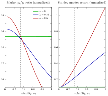
</div>

<span id="figure:changing_lambda"></span>![Figure I. Conditional moments](figures/appendix_figureI.svg)

**Figure I.** Conditional moments

<div class="minipage">

The market $p_t/y_t$ ratio (left panel) and conditional standard deviation of the market return (right panel), both as a function of the volatility state $\sigma_t$ and expressed in annual terms. Three cases are shown, the frictionless case ($\lambda=0$), our benchmark ($\lambda=0.31$), and a high segmentation case ($\lambda=0.5$). The aggregate endowment growth is fixed at its unconditional mean. The vertical dashed line is the unconditional mean $\bar{\sigma}$.
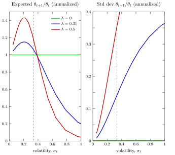
</div>

<span id="figure:theta_growth"></span>![Figure II. Multiplicative bond-pricing factor \\theta\_{t+1}/\\theta_t](figures/appendix_figureII.svg)

**Figure II.** Multiplicative bond-pricing factor $\theta_{t+1}/\theta_t$

<div class="minipage">

The expected aggregate bond-pricing factor $\theta_{t+1}/\theta_t$ (left panel) and the standard deviation of $\theta_{t+1}/\theta_t$ (right panel) as a function of the volatility state $\sigma_t$, all expressed in annual terms. Three cases are shown, the frictionless case ($\lambda=0$), our benchmark ($\lambda=0.31$), and a high segmentation case ($\lambda=0.5$). The vertical dashed line is the unconditional mean $\bar{\sigma}$.
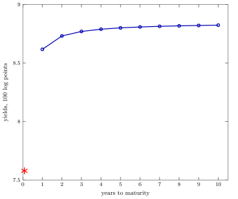
</div>

<span id="figure:AverageYieldCurve"></span>![Figure III. Average yield curve (annualized)](figures/appendix_figureIII.svg)

**Figure III.** Average yield curve (annualized)

<div class="minipage">

Average yield curve for the benchmark model. The star point on the left is the average yield on a one-month zero coupon bond, $12 \mathbb{E}\left[\log(R_f)\right]$. Note that, because the risk free rate is so volatile and because $\log(\cdot)$ is concave, this yield turns out to be about 1% lower than the average risk free rate ($R_f=8.19\%$ annual) reported in the main text.

</div>

<div id="table:handmade148455" class="paper-table">

                                                    Annualized monthly   Aggregated to yearly
  ------------------------------------------------ -------------------- ----------------------
  average real risk-free rate                              1.81                  1.81
  standard deviation of real risk free rate                1.20                  2.43
  average real NYSE return                                 7.24                  7.27
  standard deviation of real NYSE return                  14.40                 13.90
  equity premium                                           5.43                  5.47
  standard deviation of equity premium                    14.25                 13.30
  average price-dividend ratio                            495.18                34.38
  standard deviation of log price-dividend ratio           0.56                  0.34
  autocorrelation of log price-dividend ratio            $-$0.02                 0.89
  average consumption growth                               2.19                  2.17
  standard deviation of consumption growth                 1.25                  1.33

  : **Table I.** Aggregate statistics in annualized monthly data and in monthly data time-aggregated to yearly

<div class="notes">

Aggregate postwar US data. All return data is monthly 1959:1-2007:12 and reported in annualized percent. The stock market index is the value weighted NYSE return from CRSP, and the risk-free return is the 90 day T-bill rate. Real consumption growth refers to the growth of real nondurables and services consumption per capita from the BEA. The first column shows annualized statistics for monthly data. To annualize monthly returns and consumption growth, we multiply by 12, and to annualize monthly standard deviations, we multiply by $\sqrt{12}$. The second column shows statistics for yearly data, which are obtained by compounding returns and growth over the relevant time interval. The only statistics that are substantially different in this second column concern the price dividend ratio: this is because, in the first column the dividend that enters the ratio is the dividend per month, while in the second column it is the dividend paid over the entire year.

</div>

</div>

[^1]: See for example [Aiyagari and Gertler](#bib:AIYA/GERT/91) (1991), [He and Modest](#bib:HE/MODE/95) (1995) and [Luttmer](#bib:LUTT/96) (1996); [Luttmer](#bib:LUTT/99) (1999) for the quantitative evaluation of asset pricing models with trading frictions.

[^2]: Various extensions and further computational details are given in a supplementary appendix, [Edmond and Weill](#bib:EDMO/WEIL/12b) (2012), available online from the journal's website.

[^3]: [Krueger and Lustig](#bib:KRUG/LUST/08-2) (2010) also consider richer market structures, with Arrow securities paying off conditional on the realized aggregate state, and one-period riskless bonds. However, they show that there are equilibria in which there is no trade in these other markets. That is, in order to self-insure against idiosyncratic shocks, agents find it optimal to trade only aggregate endowment claims.

[^4]: See [Telmer](#bib:TELM/93-2) (1993) and [Heaton and Lucas](#bib:HEAT/LUCA/96-2) (1996) for important early applications of incomplete markets models to asset pricing.
